More Advanced Examples

Advanced examples:

• example_spintransition,

• example_spintransition_thermal,

• example_user_input_material,

• example_optimize_pv,

• example_compare_all_methods,

• example_build_planet,

• example_fit_composition,

• example_fit_data,

• example_fit_eos,

• example_fit_solution,

• example_optimal_thermobarometry,

• example_equilibrate, and

• example_olivine_binary.

example_spintransition

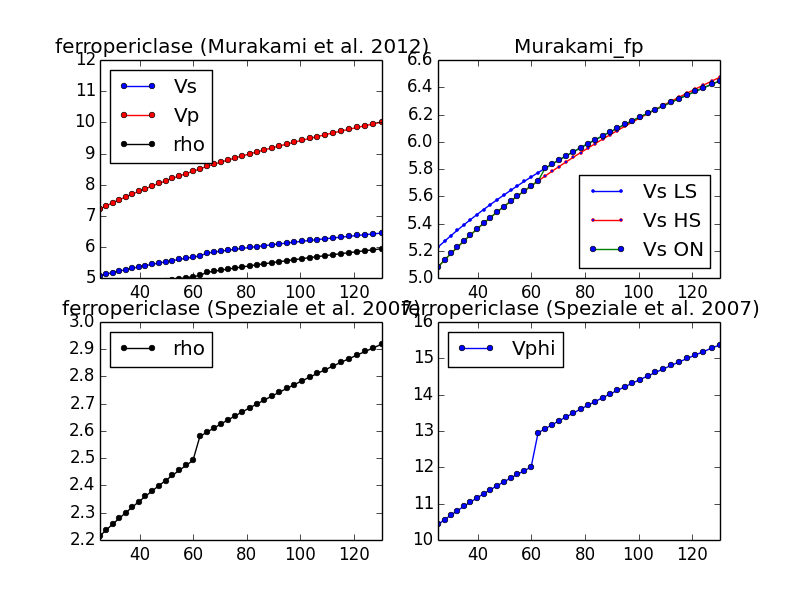
This example shows the different minerals that are implemented with a spin transition. Minerals with spin transition are implemented by defining two separate minerals (one for the low and one for the high spin state). Then a third dynamic mineral is created that switches between the two previously defined minerals by comparing the current pressure to the transition pressure.

Specifically uses:

• burnman.mineral_helpers.HelperSpinTransition()

• burnman.minerals.Murakami_etal_2012.fe_periclase()

• burnman.minerals.Murakami_etal_2012.fe_periclase_HS()

• burnman.minerals.Murakami_etal_2012.fe_periclase_LS()

Demonstrates:

• implementation of spin transition in (Mg,Fe)O at user defined pressure

Resulting figure:

example_spintransition_thermal

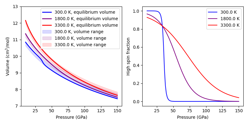
This example illustrates how to create a non-ideal solution model for (Mg,Fe^HS,Fe^LS)O ferropericlase that has a gradual spin transition at finite temperature.

In the first part of the example, we create a Solution class from scratch that incorporates three endmembers: MgO, FeO in the high spin state, and FeO in the low spin state. We then embed this solution in a RelaxedSolution class that allows us to define the isochemical high spin to low spin transition as a free relaxation vector that is allowed to vary freely to minimize the Gibbs free energy.

In the second part of the example, we illustrate how to use the ferropericlase solution model directly from the Stixrude and Lithgow-Bertelloni (2024) database, again embedding it in a RelaxedSolution to incorporate the spin transition. We then show how to calculate thermodynamic and elastic properties that incorporate the effects of the spin transition over a range of pressures and temperatures along an oceanic geotherm.

In this example, we implicitly apply the Bragg-Williams approximation (i.e., we assume that there is no short-range order by only incorporating interactions that are a function of the average occupancy of species on each distinct site). Furthermore, the implemented mixing model explicitly precludes long range order.

Specifically uses:

• burnman.Mineral

• burnman.Solution

• burnman.RelaxedSolution

Demonstrates:

• implementation of gradual spin transition in (Mg,Fe)O at a user-defined pressure and temperature

Resulting figure:

example_user_input_material

Shows user how to input a mineral of his/her choice without usint the library and which physical values need to be input for BurnMan to calculate \(V_P, V_\Phi, V_S\) and density at depth.

Specifically uses:

• burnman.Mineral

Demonstrates:

• how to create your own minerals

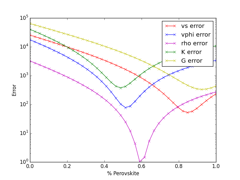
example_optimize_pv

Vary the amount perovskite vs. ferropericlase and compute the error in the seismic data against PREM. For more extensive comments on this setup, see tutorial/step_2.py

Uses:

• Mineral Datasets

• burnman.Composite

• burnman.seismic.PREM

• burnman.geotherm.BrownShankland

• burnman.Material.evaluate()

• burnman.utils.math.l2_norm_profiles()

Demonstrates:

• compare errors between models

• loops over models

Resulting figure:

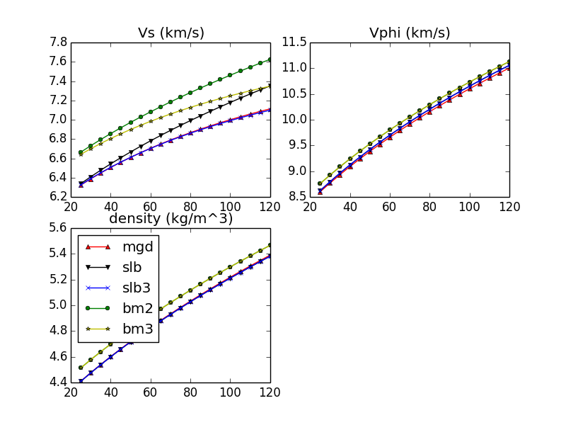
example_compare_all_methods

This example demonstrates how to call each of the individual calculation methodologies that exist within BurnMan. See below for current options. This example calculates seismic velocity profiles for the same set of minerals and a plot of \(V_s, V_\phi\) and \(\rho\) is produce for the user to compare each of the different methods.

Specifically uses:

• Equations of State for Minerals

Demonstrates:

• Each method for calculating velocity profiles currently included within BurnMan

Resulting figure:

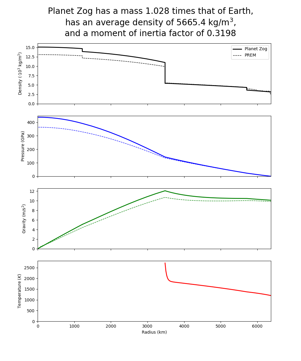
example_build_planet

For Earth we have well-constrained one-dimensional density models. This allows us to calculate pressure as a function of depth. Furthermore, petrologic data and assumptions regarding the convective state of the planet allow us to estimate the temperature.

For planets other than Earth we have much less information, and in particular we know almost nothing about the pressure and temperature in the interior. Instead, we tend to have measurements of things like mass, radius, and moment-of-inertia. We would like to be able to make a model of the planet’s interior that is consistent with those measurements.

However, there is a difficulty with this. In order to know the density of the planetary material, we need to know the pressure and temperature. In order to know the pressure, we need to know the gravity profile. And in order to the the gravity profile, we need to know the density. This is a nonlinear problem which requires us to iterate to find a self-consistent solution.

This example allows the user to define layers of planets of known outer radius and self- consistently solve for the density, pressure and gravity profiles. The calculation will iterate until the difference between central pressure calculations are less than 1e-5. The planet class in BurnMan (../burnman/planet.py) allows users to call multiple properties of the model planet after calculations, such as the mass of an individual layer, the total mass of the planet and the moment if inertia. See planets.py for information on each of the parameters which can be called.

Uses:

• Mineral Datasets

• burnman.Planet

• burnman.Layer

Demonstrates:

• setting up a planet

• computing its self-consistent state

• computing various parameters for the planet

• seismic comparison

Resulting figure:

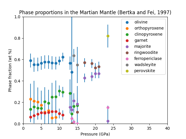
example_fit_composition

This example shows how to fit compositional data to a solution model, how to partition a bulk composition between phases of known composition, and how to assess goodness of fit.

Uses:

• burnman.Composition

• burnman.Solution

• burnman.optimize.composition_fitting.fit_phase_proportions_to_bulk_composition()

• burnman.optimize.composition_fitting.fit_composition_to_solution()

Demonstrates:

• Fitting compositional data to a solution model

• Partitioning of a bulk composition between phases of known composition

• Assessing goodness of fit.

Resulting figure:

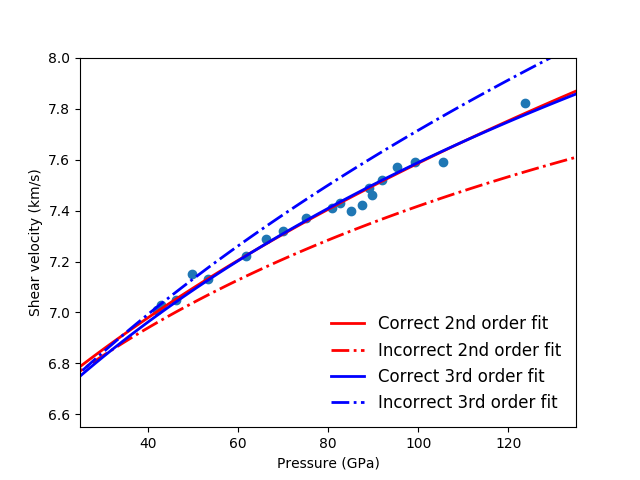
example_fit_data

This example demonstrates BurnMan’s functionality to fit various mineral physics data to an EoS of the user’s choice.

Please note also the separate file example_fit_eos.py, which can be viewed as a more advanced example in the same general field.

teaches: - least squares fitting

Resulting figures:

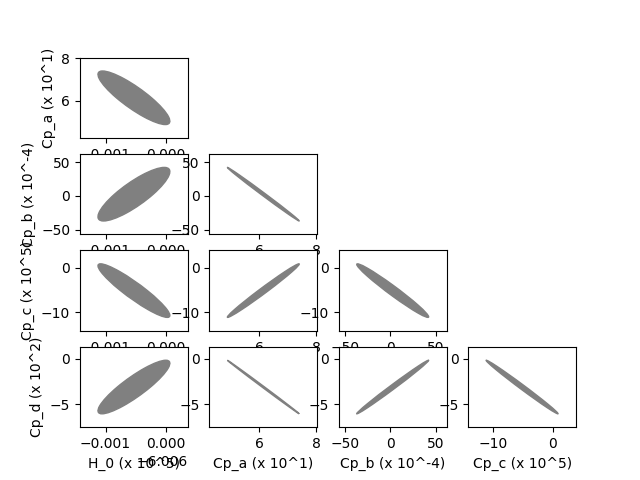
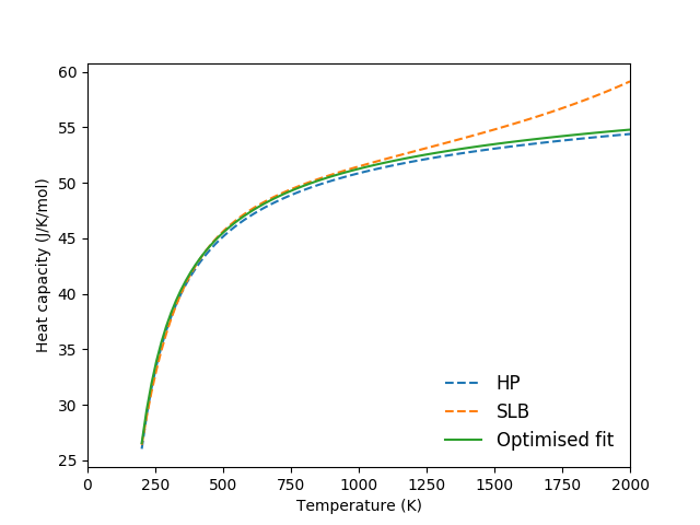
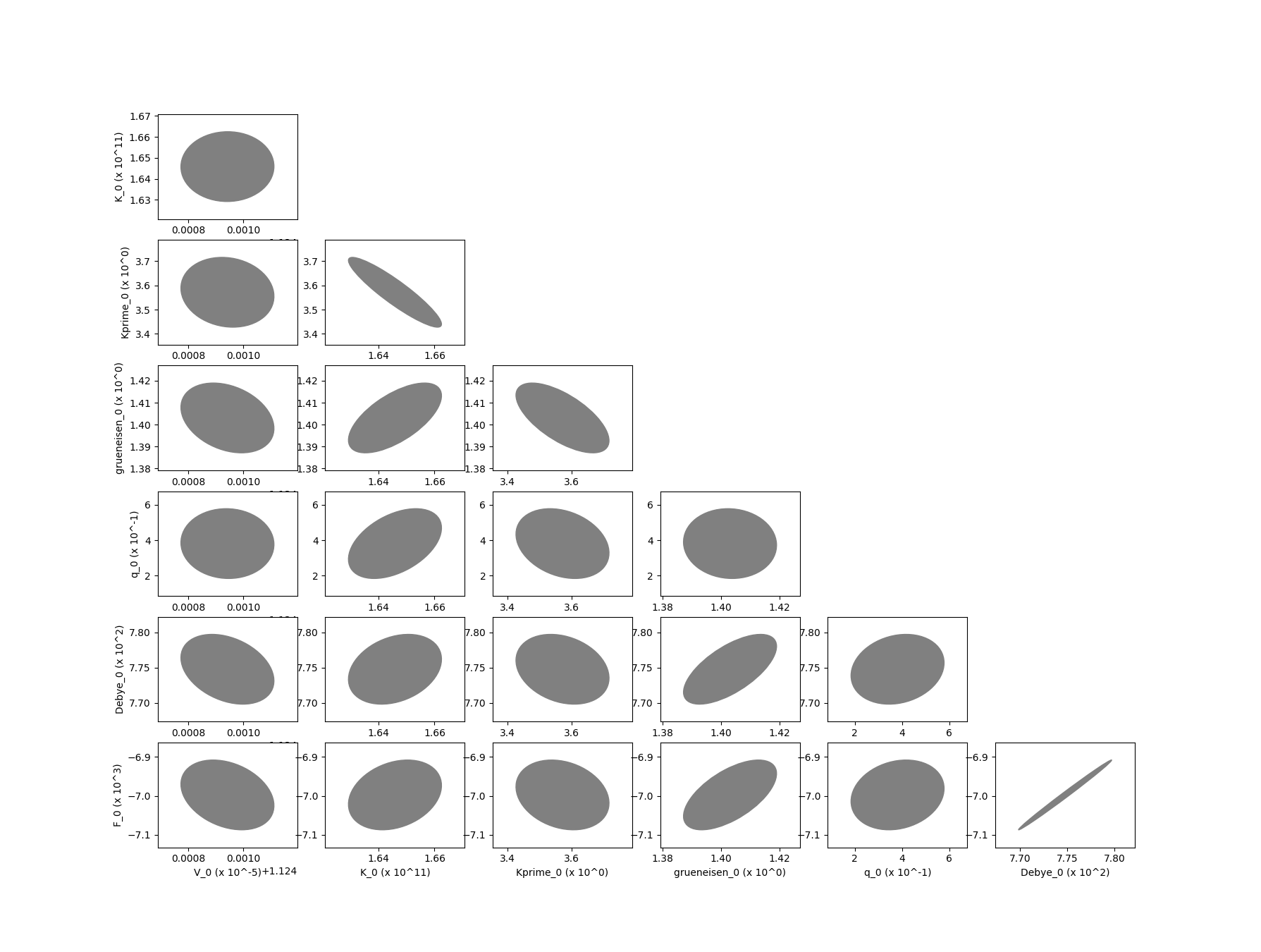
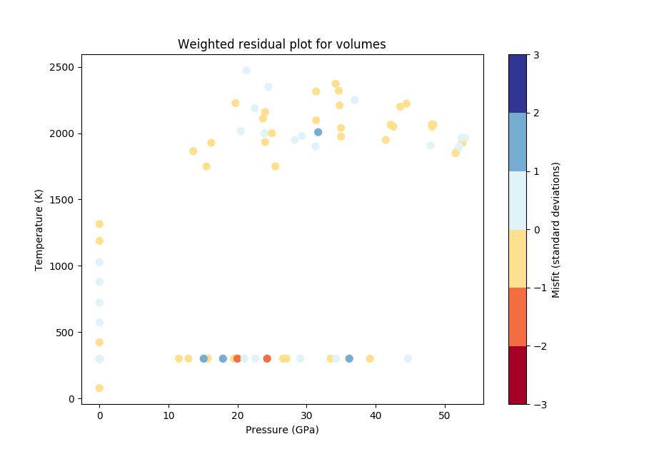
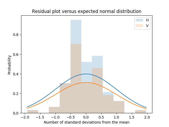
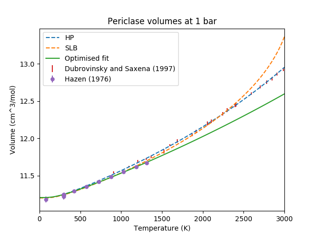
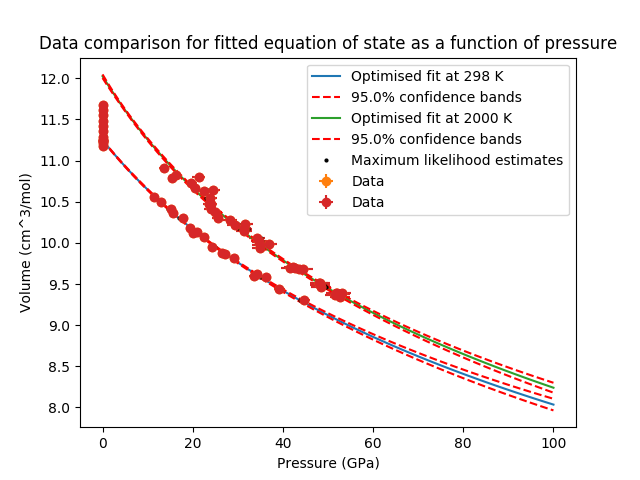
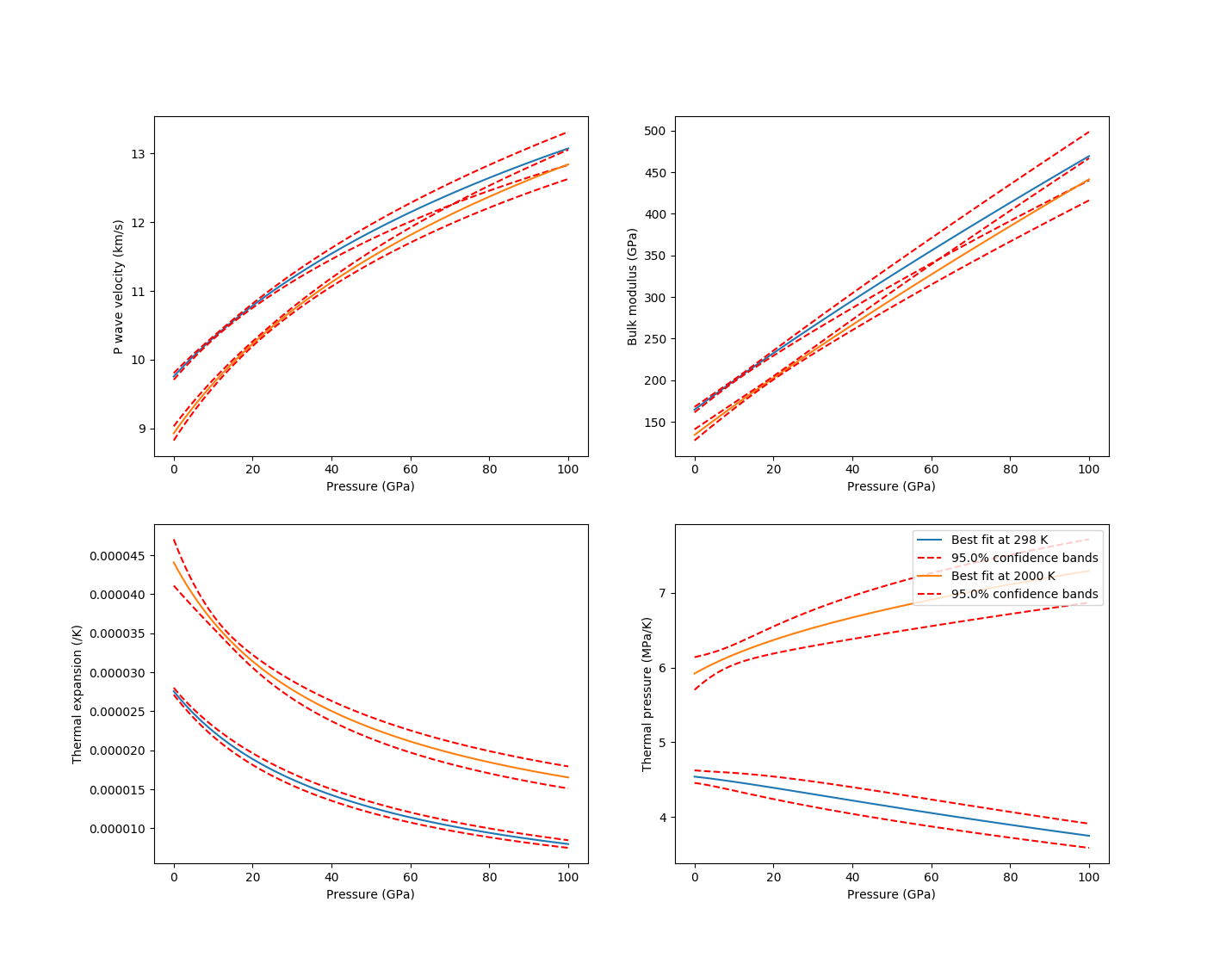
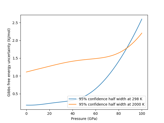
example_fit_eos

This example demonstrates BurnMan’s functionality to fit data to an EoS of the user’s choice.

The first example deals with simple PVT fitting. The second example illustrates how powerful it can be to provide non-PVT constraints to the same fitting problem.

teaches: - least squares fitting

Last seven resulting figures:

example_fit_solution

This example demonstrates how to fit parameters for solution models using a range of compositionally-variable experimental data.

The example in this file deals with finding optimized parameters for the forsterite-fayalite binary using a mixture of volume and seismic velocity data.

teaches: - least squares fitting for solution data

Resulting figures:

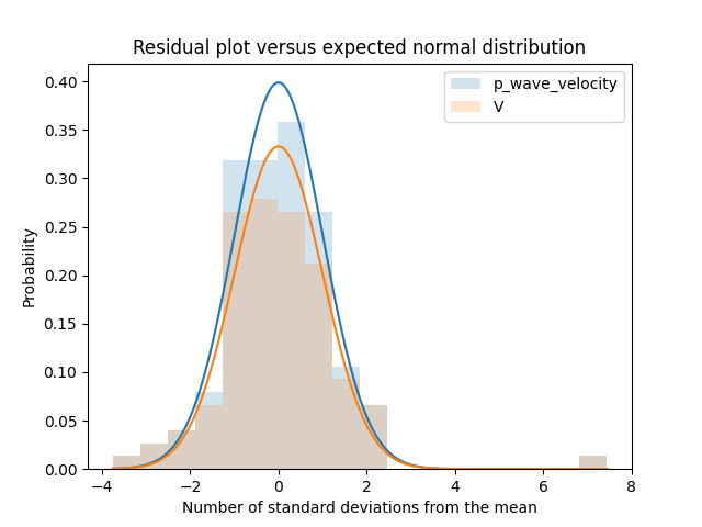
Data residuals relative to the model fitted using all the provided data.

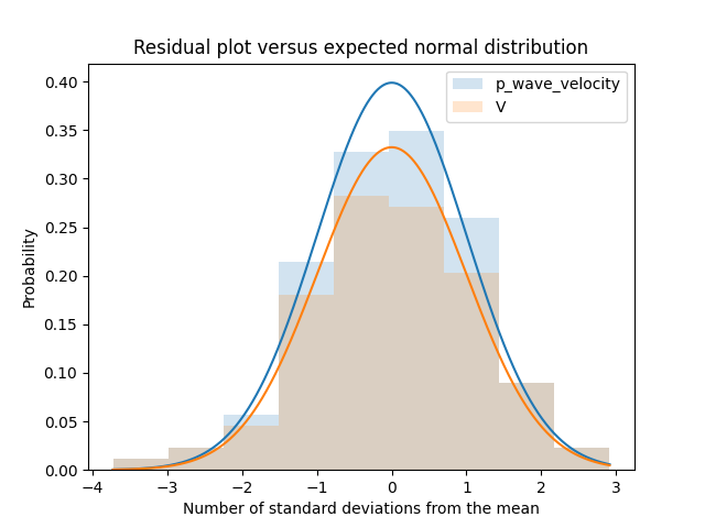
Data residuals relative to the model fitted using the provided data after semi-automatic removal of spurious data.

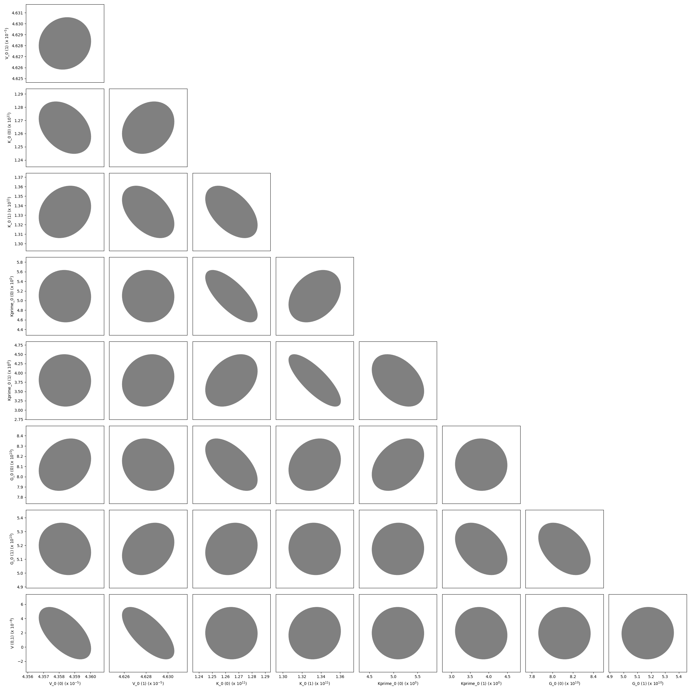
The variance-covariance matrix of the optimized parameters shown as a corner plot.

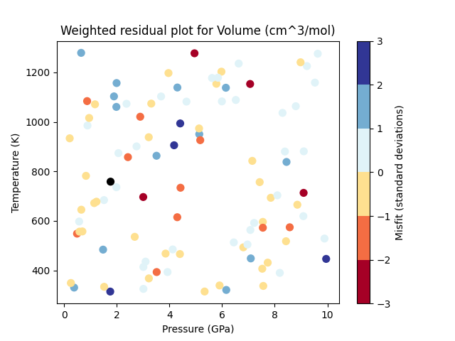
A P-T plot showing the weighted residuals of each piece of volume data.

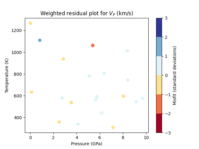
A P-T plot showing the weighted residuals of each piece of P-wave velocity data.

example_equilibrate

This example demonstrates how BurnMan may be used to calculate the equilibrium state for an assemblage of a fixed bulk composition given two constraints. Each constraint has the form [<constraint type>, <constraint>], where <constraint type> is one of the strings: P, T, S, V, X, PT_ellipse, phase_fraction, or phase_composition. The <constraint> object should either be a float or an array of floats for P, T, S, V (representing the desired pressure, temperature, entropy or volume of the material). If the constraint type is X (a generic constraint on the solution vector) then the constraint c is represented by the following equality: np.dot(c[0], x) - c[1]. If the constraint type is PT_ellipse, the equality is given by norm(([P, T] - c[0])/c[1]) - 1. The constraint_type phase_fraction assumes a tuple of the phase object (which must be one of the phases in the burnman.Composite) and a float or vector corresponding to the phase fractions. Finally, a phase_composition constraint has the format (site_names, n, d, v), where site names dictates the sites involved in the equality constraint. The equality constraint is given by n*x/d*x = v, where x are the site occupancies and n and d are fixed vectors of site coefficients. So, one could for example choose a constraint ([Mg_A, Fe_A], [1., 0.], [1., 1.], [0.5]) which would correspond to equal amounts Mg and Fe on the A site.

This script provides a number of examples, which can be turned on and off with a series of boolean variables. In order of complexity:

• run_aluminosilicates: Creates the classic aluminosilicate diagram involving univariate reactions between andalusite, sillimanite and kyanite.

• run_ordering: Calculates the state of order of Jennings and Holland (2015) orthopyroxene in the simple en-fs binary at 1 bar.

• run_gt_solvus: Demonstrates the shape of the pyrope-grossular solvus.

• run_fper_ol: Calculates the equilibrium Mg-Fe partitioning between ferropericlase and olivine.

• run_fixed_ol_composition: Calculates the composition of wadsleyite in equilibrium with olivine of a fixed composition at a fixed pressure.

• run_upper_mantle: Calculates the equilibrium compositions and phase proportions for an ol-opx-gt composite in an NCFMAS bulk composition.

• run_lower_mantle: Calculates temperatures and assemblage properties along an isentrope in the lower mantle. Includes calculations of the post-perovskite-in and bridgmanite-out lines.

• run_olivine_polymorphs: Produces a P-T pseudosection for a fo90 composition.

Uses:

• Mineral Datasets

• burnman.Composite

• burnman.equilibrate()

Resulting figures:

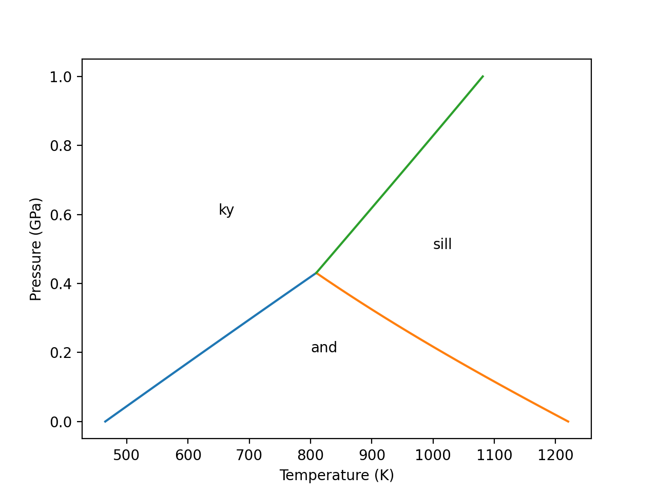
The classic aluminosilicate diagram.

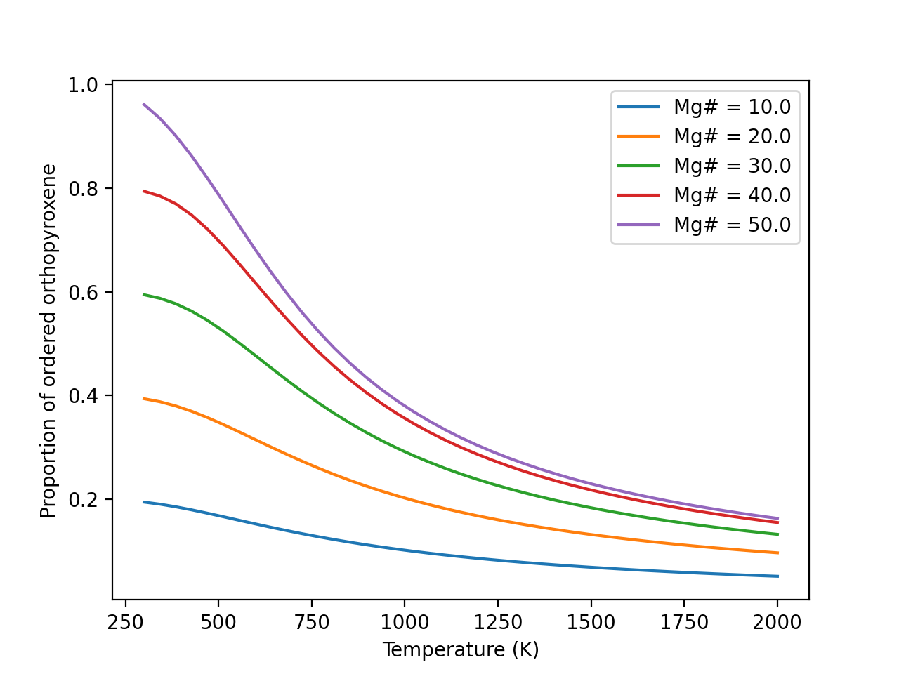
Ordering in two site orthopyroxene.

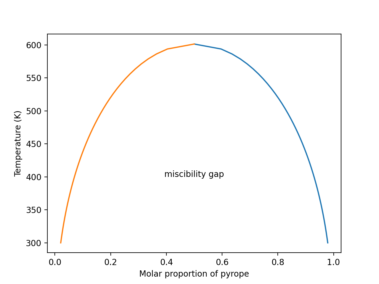
Miscibility in the pyrope-grossular garnet system

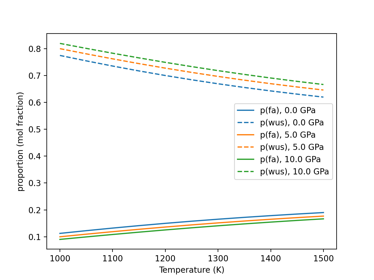
Mg-Fe partitioning between olivine and ferropericlase.

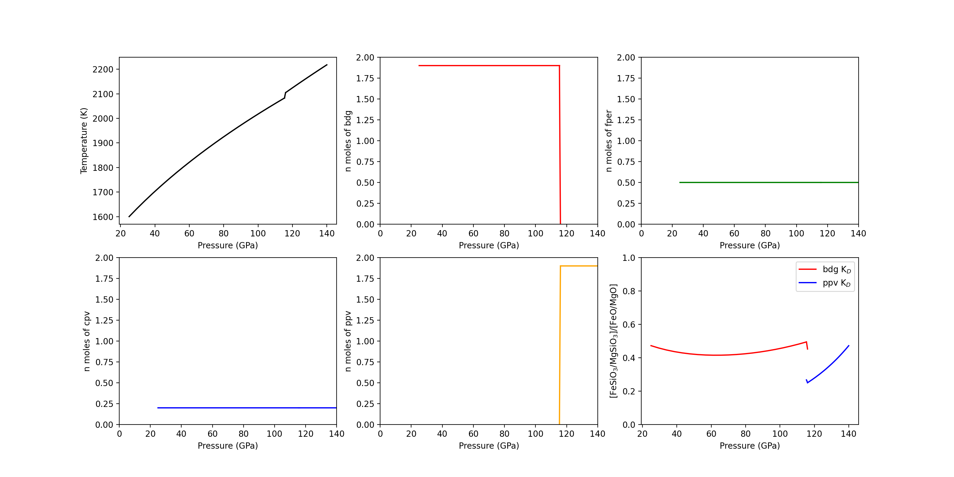
Phase equilibria in the lower mantle.

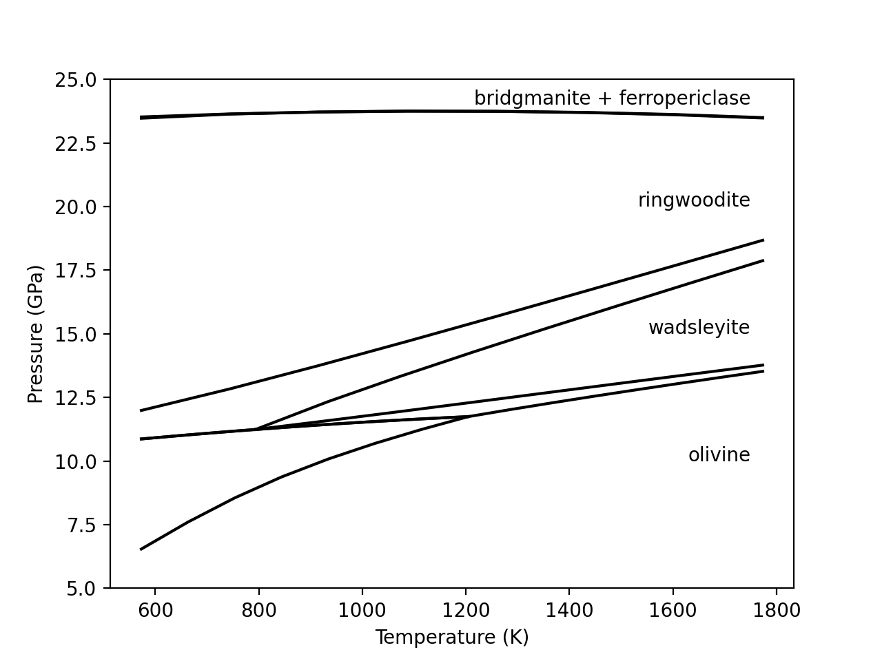
A P-T pseudosection for a composition of Fe0.2Mg1.8SiO4 (fo90).

example_olivine_binary

This example demonstrates how BurnMan may be used to calculate the equilibrium binary phase diagram for the three olivine polymorphs (olivine, wadsleyite and ringwoodite).

The calculations use the equilibrate function. Unlike the examples in example_equilibrate.py, which are constrained to a fixed bulk composition, the bulk composition is allowed to vary along the vector [n_Mg - n_Fe].

Uses:

• Mineral Datasets

• burnman.Composite

• burnman.equilibrate()

Resulting figures:

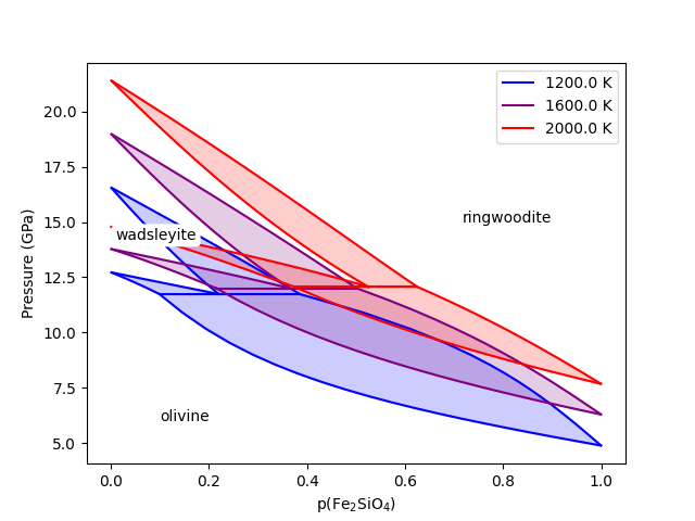
The olivine polymorph binary phase diagram using the thermodynamic models of Stixrude and Lithgow-Bertelloni (2011).