The BurnMan Tutorial
Part 4: Fitting#
This file is part of BurnMan - a thermoelastic and thermodynamic toolkit for the Earth and Planetary Sciences
Copyright (C) 2012 - 2021 by the BurnMan team, released under the GNU GPL v2 or later.
Introduction#
This ipython notebook is the fourth in a series designed to introduce new users to the code structure and functionalities present in BurnMan.
Demonstrates
burnman.optimize.eos_fitting.fit_PTV_data
burnman.optimize.composition_fitting.fit_composition_to_solution
burnman.optimize.composition_fitting.fit_phase_proportions_to_bulk_composition
Everything in BurnMan and in this tutorial is defined in SI units.
[1]:
import burnman
import numpy as np
import matplotlib.pyplot as plt
Warning: No module named 'cdd'. For full functionality of BurnMan, please install pycddlib.
Fitting parameters for an equation of state to experimental data#
BurnMan contains least-squares optimization functions that fit model parameters to data. There are two helper functions especially for use in fitting Mineral parameters to experimental data; these are burnman.optimize.eos_fitting.fit_PTp_data (which can fit multiple kinds of data at the same time), and burnman.optimize.eos_fitting.fit_PTV_data, which specifically fits only pressure-temperature-volume data.
An extended example of fitting various kinds of data, outlier removal and detailed analysis can be found in examples/example_fit_eos.py. In this tutorial, we shall focus solely on fitting room temperature pressure-temperature-volume data. Specifically, the data we will fit is experimental volumes of stishovite, taken from Andrault et al. (2003). This data is provided in the form [P (GPa), V (Angstrom^3) and sigma_V (Angstrom^3)].
[2]:
PV = np.array([[0.0001, 46.5126, 0.0061],
               [1.168, 46.3429, 0.0053],
               [2.299, 46.1756, 0.0043],
               [3.137, 46.0550, 0.0051],
               [4.252, 45.8969, 0.0045],
               [5.037, 45.7902, 0.0053],
               [5.851, 45.6721, 0.0038],
               [6.613, 45.5715, 0.0050],
               [7.504, 45.4536, 0.0041],
               [8.264, 45.3609, 0.0056],
               [9.635, 45.1885, 0.0042],
               [11.69, 44.947, 0.002],
               [17.67, 44.264, 0.002],
               [22.38, 43.776, 0.003],
               [29.38, 43.073, 0.009],
               [37.71, 42.278, 0.008],
               [46.03, 41.544, 0.017],
               [52.73, 40.999, 0.009],
               [26.32, 43.164, 0.006],
               [30.98, 42.772, 0.005],
               [34.21, 42.407, 0.003],
               [38.45, 42.093, 0.004],
               [43.37, 41.610, 0.004],
               [47.49, 41.280, 0.007]])

print(f'{len(PV)} data points loaded successfully.')
24 data points loaded successfully.
BurnMan works exclusively in SI units, so we have to convert from GPa to Pa, and Angstrom per cell into molar volume in m^3. The fitting function also takes covariance matrices as input, so we have to build those matrices.
[3]:
from burnman.tools.unitcell import molar_volume_from_unit_cell_volume

Z = 2. # number of formula units per unit cell in stishovite
PTV = np.array([PV[:,0]*1.e9,
                298.15 * np.ones_like(PV[:,0]),
                molar_volume_from_unit_cell_volume(PV[:,1], Z)]).T

# Here, we assume that the pressure uncertainties are equal to 3% of the total pressure,
# that the temperature uncertainties are negligible, and take the unit cell volume
# uncertainties from the paper.
# We also assume that the uncertainties in pressure and volume are uncorrelated.
nul = np.zeros_like(PTV[:,0])
PTV_covariances = np.array([[0.03*PTV[:,0], nul, nul],
                            [nul, nul, nul],
                            [nul, nul, molar_volume_from_unit_cell_volume(PV[:,2], Z)]]).T
PTV_covariances = np.power(PTV_covariances, 2.)
The next code block creates a Mineral object (stv), providing starting guesses for the parameters. The user selects which parameters they wish to fit, and which they wish to keep fixed. The parameters of the Mineral object are automatically updated during fitting.
Finally, the optimized parameter values and their variances are printed to screen.
[4]:
stv = burnman.minerals.HP_2011_ds62.stv()
params = ['V_0', 'K_0', 'Kprime_0']
fitted_eos = burnman.optimize.eos_fitting.fit_PTV_data(stv, params, PTV, PTV_covariances, verbose=False)

print('Optimized equation of state for stishovite:')
burnman.utils.misc.pretty_print_values(fitted_eos.popt, fitted_eos.pcov, fitted_eos.fit_params)
print('')
Optimized equation of state for stishovite:
V_0: (1.4005 +/- 0.0001) x 1e-05
K_0: (3.12 +/- 0.03) x 1e+11
Kprime_0: (4.4 +/- 0.2) x 1e+00
The fitted_eos object contains a lot of useful information about the fit. In the next code block, we fit the corner plot of the covariances, showing the tradeoffs in different parameters.
[5]:
import matplotlib
matplotlib.rc('axes.formatter', useoffset=False) # turns offset off, makes for a more readable plot

fig = burnman.nonlinear_fitting.corner_plot(fitted_eos.popt, fitted_eos.pcov,
                                            params)
axes = fig[1]
axes[1][0].set_xlabel('$V_0$ ($\\times 10^{-5}$ m$^3$)')
axes[1][1].set_xlabel('$K_0$ ($\\times 10^{11}$ Pa)')
axes[0][0].set_ylabel('$K_0$ ($\\times 10^{11}$ Pa)')
axes[1][0].set_ylabel('$K\'_0$')
plt.show()
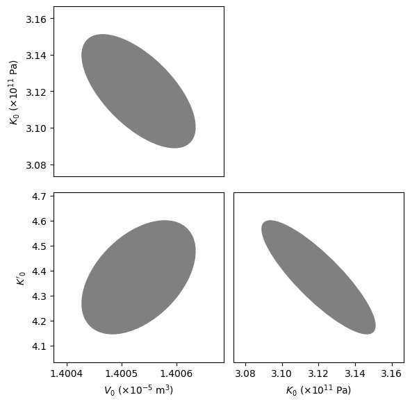
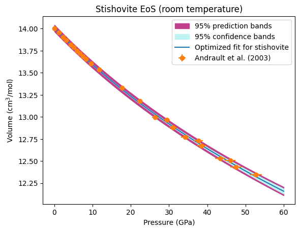
We now plot our optimized equation of state against the original data. BurnMan also includes a useful function burnman.optimize.nonlinear_fitting.confidence_prediction_bands that can be used to calculate the nth percentile confidence and prediction bounds on a function given a model using the delta method.
[6]:
from burnman.utils.misc import attribute_function
from burnman.optimize.nonlinear_fitting import confidence_prediction_bands

T = 298.15
pressures = np.linspace(1.e5, 60.e9, 101)
temperatures = T*np.ones_like(pressures)
volumes = stv.evaluate(['V'], pressures, temperatures)[0]
PTVs = np.array([pressures, temperatures, volumes]).T

# Calculate the 95% confidence and prediction bands
cp_bands = confidence_prediction_bands(model=fitted_eos,
                                       x_array=PTVs,
                                       confidence_interval=0.95,
                                       f=attribute_function(stv, 'V'),
                                       flag='V')

plt.fill_between(pressures/1.e9, cp_bands[2] * 1.e6, cp_bands[3] * 1.e6,
                 color=[0.75, 0.25, 0.55], label='95% prediction bands')
plt.fill_between(pressures/1.e9, cp_bands[0] * 1.e6, cp_bands[1] * 1.e6,
                 color=[0.75, 0.95, 0.95], label='95% confidence bands')

plt.plot(PTVs[:,0] / 1.e9, PTVs[:,2] * 1.e6, label='Optimized fit for stishovite')
plt.errorbar(PTV[:,0] / 1.e9, PTV[:,2] * 1.e6,
             xerr=np.sqrt(PTV_covariances[:,0,0]) / 1.e9,
             yerr=np.sqrt(PTV_covariances[:,2,2]) * 1.e6,
             linestyle='None', marker='o', label='Andrault et al. (2003)')

plt.ylabel("Volume (cm$^3$/mol)")
plt.xlabel("Pressure (GPa)")
plt.legend(loc="upper right")
plt.title("Stishovite EoS (room temperature)")
plt.show()
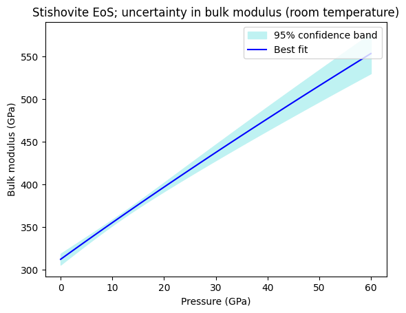
We can also calculate the confidence and prediction bands for any other property of the mineral. In the code block below, we calculate and plot the optimized isothermal bulk modulus and its uncertainties.
[7]:
cp_bands = confidence_prediction_bands(model=fitted_eos,
                                       x_array=PTVs,
                                       confidence_interval=0.95,
                                       f=attribute_function(stv, 'K_T'),
                                       flag='V')

plt.fill_between(pressures/1.e9, (cp_bands[0])/1.e9, (cp_bands[1])/1.e9, color=[0.75, 0.95, 0.95], label='95% confidence band')
plt.plot(pressures/1.e9, (cp_bands[0] + cp_bands[1])/2.e9, color='b', label='Best fit')

plt.ylabel("Bulk modulus (GPa)")
plt.xlabel("Pressure (GPa)")
plt.legend(loc="upper right")
plt.title("Stishovite EoS; uncertainty in bulk modulus (room temperature)")
plt.show()
Finding the best fit endmember proportions of a solution given a bulk composition#
Let’s now turn our focus to a different kind of fitting. It is common in petrology to have a bulk composition of a phase (provided, for example, by electron probe microanalysis), and want to turn this composition into a formula that satisfies stoichiometric constraints. This can be formulated as a constrained, weighted least squares problem, and BurnMan can be used to solve these problems using the function burnman.optimize.composition_fitting.fit_composition_to_solution.
In the following example, we shall create a model garnet composition, and then fit that to the Jennings and Holland (2015) garnet solution model. First, let’s look at the solution model endmembers (pyrope, almandine, grossular, andradite and knorringite):
[8]:
from burnman import minerals

gt = minerals.JH_2015.garnet()

print(f'Endmembers: {gt.endmember_names}')
print(f'Elements: {gt.elements}')
print('Stoichiometric matrix:')
print(gt.stoichiometric_matrix)
Endmembers: ['py', 'alm', 'gr', 'andr', 'knor']
Elements: ['Ca', 'Mg', 'Cr', 'Fe', 'Al', 'Si', 'O']
Stoichiometric matrix:
Matrix([[0, 3, 0, 0, 2, 3, 12], [0, 0, 0, 3, 2, 3, 12], [3, 0, 0, 0, 2, 3, 12], [3, 0, 0, 2, 0, 3, 12], [0, 3, 2, 0, 0, 3, 12]])
Now, let’s create a model garnet composition. A unique composition can be determined with the species Fe (total), Ca, Mg, Cr, Al, Si and Fe3+, all given in mole amounts. On top of this, we add some random noise (using a fixed seed so that the composition is reproducible).
[9]:
fitted_variables = ['Fe', 'Ca', 'Mg', 'Cr', 'Al', 'Si', 'Fe3+']
variable_values = np.array([1.1, 2., 0., 0, 1.9, 3., 0.1])
variable_covariances = np.eye(7)*0.01*0.01

# Add some noise.
v_err = np.random.rand(7)
np.random.seed(100)
variable_values = np.random.multivariate_normal(variable_values,
                                                variable_covariances)
Importantly, Fe3+ isn’t an element or a site-species of the solution model, so we need to provide the linear conversion from Fe3+ to elements and/or site species. In this case, Fe3+ resides only on the second site (Site B), and the JH_2015.gt model has labelled Fe3+ on that site as Fef. Therefore, the conversion is simply Fe3+ = Fef_B.
[10]:
variable_conversions = {'Fe3+': {'Fef_B': 1.}}
Now we’re ready to do the fitting. The following line is all that is required, and yields as output the optimized parameters, the corresponding covariance matrix and the residual.
[11]:
from burnman.optimize.composition_fitting import fit_composition_to_solution
popt, pcov, res = fit_composition_to_solution(gt,
                                              fitted_variables,
                                              variable_values,
                                              variable_covariances,
                                              variable_conversions)
Finally, the optimized parameters can be used to set the composition of the solution model, and the optimized parameters printed to stdout.
[12]:
# We can set the composition of gt using the optimized parameters
gt.set_composition(popt)

# Print the optimized parameters and principal uncertainties
print('Molar fractions:')
for i in range(len(popt)):
    print(f'{gt.endmember_names[i]}: '
            f'{gt.molar_fractions[i]:.3f} +/- '
            f'{np.sqrt(pcov[i][i]):.3f}')

print(f'Weighted residual: {res:.3f}')
Molar fractions:
py: 0.004 +/- 0.005
alm: 0.328 +/- 0.003
gr: 0.619 +/- 0.004
andr: 0.048 +/- 0.004
knor: 0.000 +/- 0.004
Weighted residual: 0.519
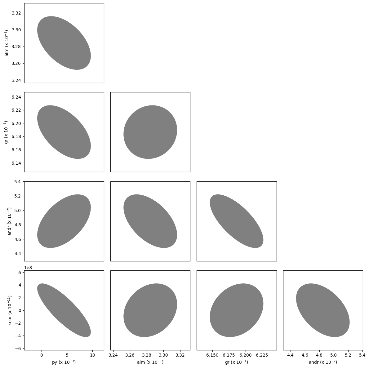
As in the equation of state fitting, a corner plot of the covariances can also be plotted.
[13]:
fig = burnman.nonlinear_fitting.corner_plot(popt, pcov, gt.endmember_names)
Fitting phase proportions to a bulk composition#
Another common constrained weighted least squares problem involves fitting phase proportions, given their individual compositions and the overall bulk composition. This is particularly important in experimental petrology, where the bulk composition is known from a starting composition. In these cases, the residual after fitting is often used to assess whether the sample remained a closed system during the experiment.
In the following example, we take phase compositions and the bulk composition reported from high pressure experiments on a Martian mantle composition by Bertka and Fei (1997), and use these to calculate phase proportions in Mars mantle, and the quality of the experiments.
First, some tedious data preparation…
[14]:
import itertools

# Load and transpose input data
filename = '../burnman/data/input_fitting/Bertka_Fei_1997_mars_mantle.dat'
with open(filename) as f:
    column_names = f.readline().strip().split()[1:]
data = np.genfromtxt(filename, dtype=None, encoding='utf8')
data = list(map(list, itertools.zip_longest(*data, fillvalue=None)))

# The first six columns are compositions given in weight % oxides
compositions = np.array(data[:6])

# The first row is the bulk composition
bulk_composition = compositions[:, 0]

# Load all the data into a dictionary
data = {column_names[i]: np.array(data[i])
        for i in range(len(column_names))}

# Make ordered lists of samples (i.e. experiment ID) and phases
samples = []
phases = []
for i in range(len(data['sample'])):
    if data['sample'][i] not in samples:
        samples.append(data['sample'][i])
    if data['phase'][i] not in phases:
        phases.append(data['phase'][i])

samples.remove("bulk_composition")
phases.remove("bulk")

# Get the indices of all the phases present in each sample
sample_indices = [[i for i in range(len(data['sample']))
                    if data['sample'][i] == sample]
                    for sample in samples]

# Get the run pressures of each experiment
pressures = np.array([data['pressure'][indices[0]] for indices in sample_indices])
The following code block loops over each of the compositions, and finds the best weight proportions and uncertainties on those proportions.
[15]:
from burnman.optimize.composition_fitting import fit_phase_proportions_to_bulk_composition

# Create empty arrays to store the weight proportions of each phase,
# and the principal uncertainties (we do not use the covariances here,
# although they are calculated)
weight_proportions = np.zeros((len(samples), len(phases)))*np.NaN
weight_proportion_uncertainties = np.zeros((len(samples),
                                            len(phases)))*np.NaN

residuals = []
# Loop over the samples, fitting phase proportions
# to the provided bulk composition
for i, sample in enumerate(samples):
    # This line does the heavy lifting
    popt, pcov, res = fit_phase_proportions_to_bulk_composition(compositions[:, sample_indices[i]],
                                                                bulk_composition)

    residuals.append(res)

    # Fill the correct elements of the weight_proportions
    # and weight_proportion_uncertainties arrays
    sample_phases = [data['phase'][i] for i in sample_indices[i]]
    for j, phase in enumerate(sample_phases):
        weight_proportions[i, phases.index(phase)] = popt[j]
        weight_proportion_uncertainties[i, phases.index(phase)] = np.sqrt(pcov[j][j])
Finally, we plot the data.
[16]:
fig = plt.figure(figsize=(6, 5))
ax = [fig.add_subplot(3, 1, 1)]
ax.append(fig.add_subplot(3, 1, (2, 4)))
for i, phase in enumerate(phases):
    ebar = plt.errorbar(pressures, weight_proportions[:, i],
                        yerr=weight_proportion_uncertainties[:, i],
                        fmt="none", zorder=2)
    ax[1].scatter(pressures, weight_proportions[:, i], label=phase, zorder=3)

ax[0].set_title('Phase proportions in the Martian Mantle (Bertka and Fei, 1997)')
ax[0].scatter(pressures, residuals)
for i in range(2):
    ax[i].set_xlim(0., 40.)

ax[1].set_ylim(0., 1.)
ax[0].set_ylabel('Residual')
ax[1].set_xlabel('Pressure (GPa)')
ax[1].set_ylabel('Phase fraction (wt)')
ax[1].legend()
fig.set_tight_layout(True)
plt.show()
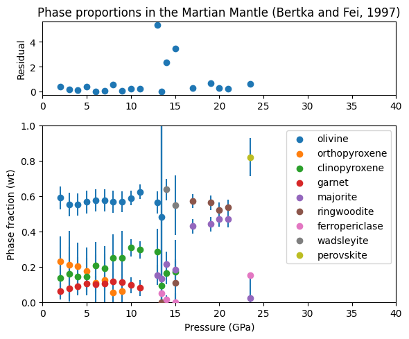
We can see from this plot that most of the residuals are below one, indicating that the probe analyses consistent with the bulk composition. Three analyses have higher residuals, which may indicate a problem with the experiments, or with the analyses around the wadsleyite field.
The phase proportions also show some nice trends; clinopyroxene weight percentage increases with pressure at the expense of orthopyroxene. Garnet / majorite percentage increases sharply as clinopyroxene is exhausted at 14-16 GPa.
And we’re done! Next time, we’ll look at how to determine equilibrium assemblages in BurnMan.