Simple Examples
- The following is a list of simple examples:
example_beginner
This example script is intended for absolute beginners to BurnMan. We cover importing BurnMan modules, creating a composite material, and calculating its seismic properties at lower mantle pressures and temperatures. Afterwards, we plot it against a 1D seismic model for visual comparison.
Uses:
burnman.seismic.PREMburnman.geotherm.BrownShankland
Demonstrates:
creating basic composites
calculating thermoelastic properties
seismic comparison
Resulting figure:
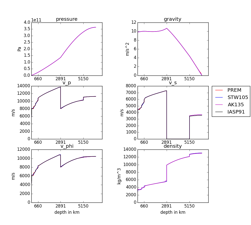
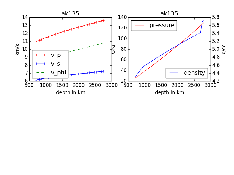
example_seismic
Shows the various ways to input seismic models (\(V_s, V_p, V_{\phi}, \rho\)) as a function of depth (or pressure) as well as different velocity model libraries available within Burnman:
This example will first calculate or read in a seismic model and plot the model along the defined pressure range. The example also illustrates how to import a seismic model of your choice, here shown by importing AK135 [KEB95].
Uses:
Demonstrates:
Utilization of library seismic models within BurnMan
Input of user-defined seismic models
Resulting figures:
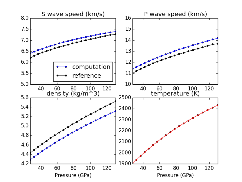
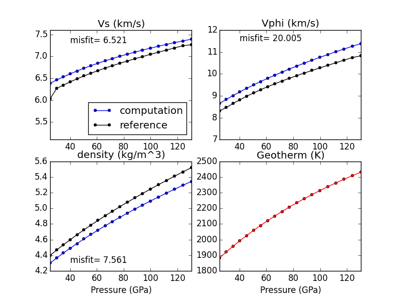
example_composite_seismic_velocities
This example shows how to create different minerals, how to compute seismic velocities, and how to compare them to a seismic reference model.
There are many different ways in BurnMan to combine minerals into a composition. Here we present a couple of examples:
Two minerals mixed in simple mole fractions. Can be chosen from the BurnMan libraries or from user defined minerals (see example_user_input_material)
Example with three minerals
Using preset solutions
Defining your own solution
To turn a method of mineral creation “on” the first if statement above the method must be set to True, with all others set to False.
Note: These minerals can include a spin transition in (Mg,Fe)O, see example_spintransition.py for explanation of how to implement this
Uses:
Demonstrates:
Different ways to define a composite
Using minerals and solutions
Compare computations to seismic models
Resulting figure:
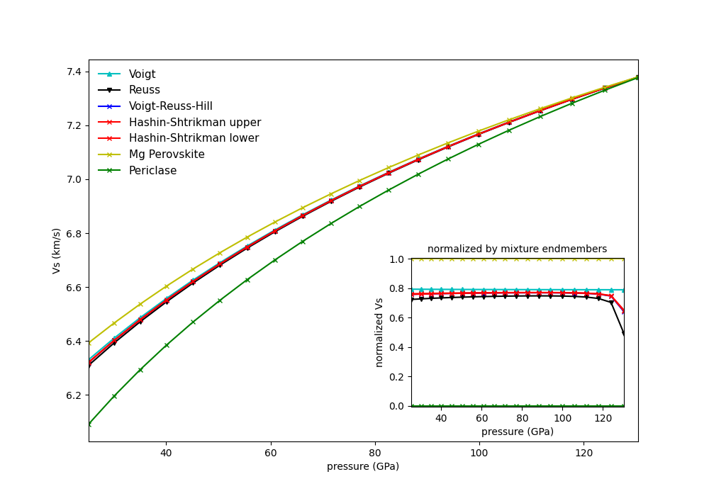
example_averaging
This example shows the effect of different averaging schemes. Currently four averaging schemes are available:
Voigt-Reuss-Hill
Voigt averaging
Reuss averaging
Hashin-Shtrikman averaging
See [WDOConnell76] Journal of Geophysics and Space Physics for explanations of each averaging scheme.
Specifically uses:
Demonstrates:
implemented averaging schemes
Resulting figure:
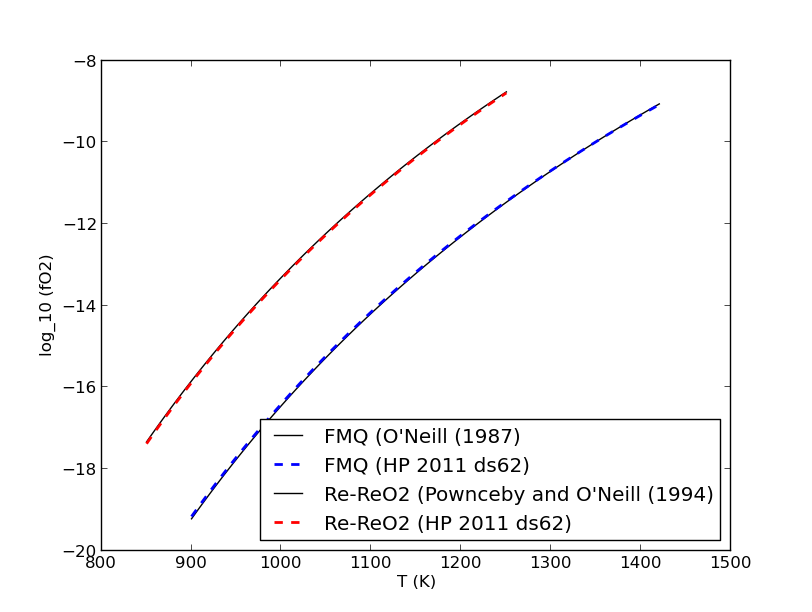
example_chemical_potentials
This example shows how to obtain chemical potentials and associated properties from an assemblage.
Demonstrates:
How to calculate chemical potentials of an assemblage.
How to compute fugacities and relative fugacities.
Resulting figure: