Class examples
The following is a list of examples that introduce the main classes of BurnMan objects:
example_geotherms, andexample_mineral
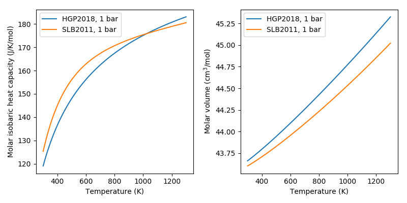
This example shows how to create mineral objects in BurnMan, and how to output their thermodynamic and thermoelastic quantities.
Mineral objects are the building blocks for more complex objects in BurnMan. These objects are intended to represent minerals (or melts, or fluids) of fixed composition, with a well defined equation of state that defines the relationship between the current state (pressure and temperature) of the mineral and its thermodynamic potentials and derivatives (such as volume and entropy).
Mineral objects are initialized with a dictionary containing all of the parameters required by the desired equation of state. BurnMan contains implementations of may equations of state (Equations of State for Minerals).
Uses:
Demonstrates:
Different ways to define an endmember
How to set state
How to output thermodynamic and thermoelastic properties
Resulting figure:
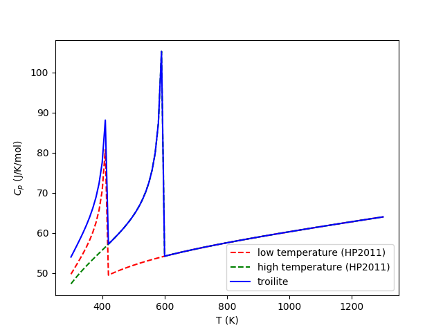
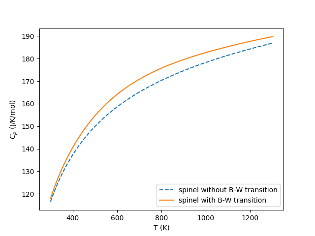
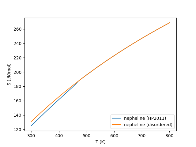
example_gibbs_modifiers
This example script demonstrates the modifications to the gibbs free energy (and derivatives) that can be applied as masks over the results from the equations of state.
These modifications currently take the forms:
Landau corrections (implementations of Putnis (1992) and Holland and Powell (2011)
Bragg-Williams corrections (implementation of Holland and Powell (1996))
Linear (a simple delta_E + delta_V*P - delta_S*T
Magnetic (Chin, Hertzman and Sundman (1987))
Uses:
Demonstrates:
creating a mineral with excess contributions
calculating thermodynamic properties
Resulting figures:
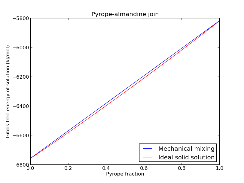
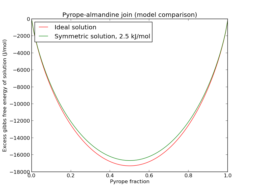
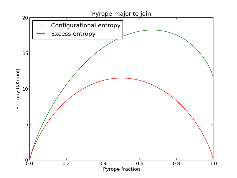
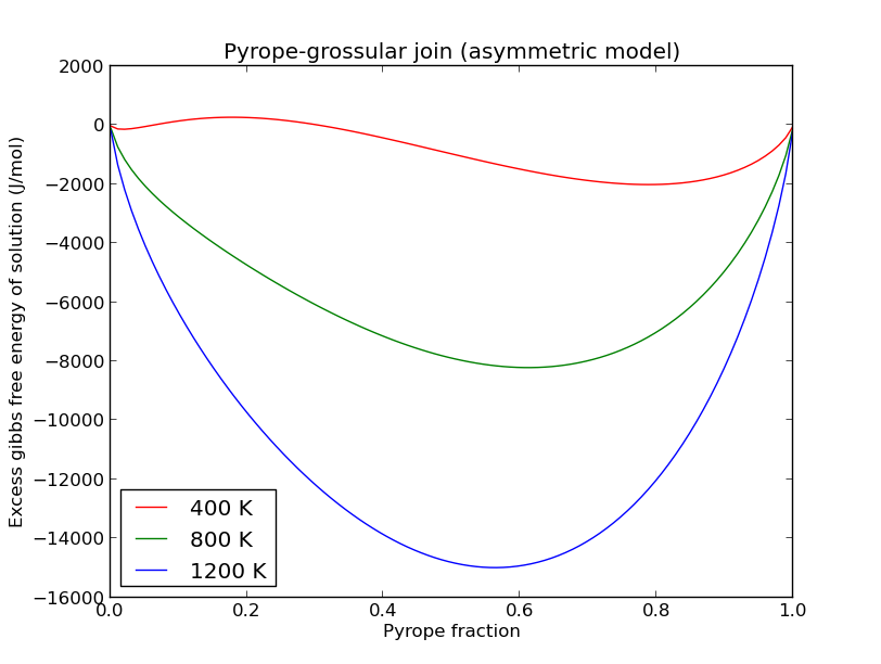
example_solution
This example shows how to create different solution models and output thermodynamic and thermoelastic quantities.
There are four main types of solution currently implemented in BurnMan:
Ideal solutions
Symmmetric solutions
Asymmetric solutions
Subregular solutions
These solutions can potentially deal with:
Disordered endmembers (more than one element on a crystallographic site)
Site vacancies
More than one valence/spin state of the same element on a site
Uses:
Demonstrates:
Different ways to define a solution
How to set composition and state
How to output thermodynamic and thermoelastic properties
Resulting figures:
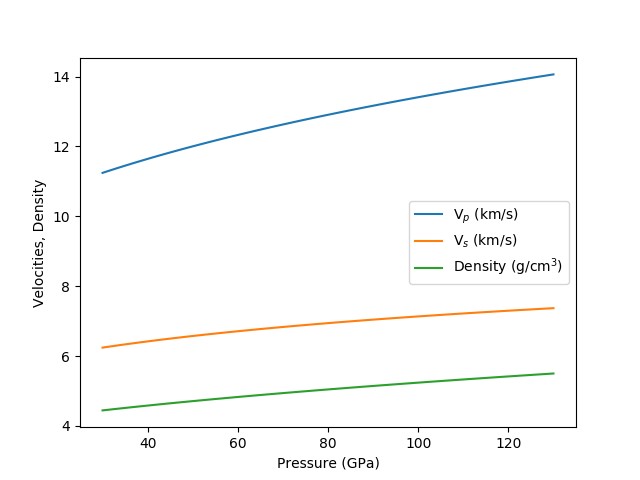
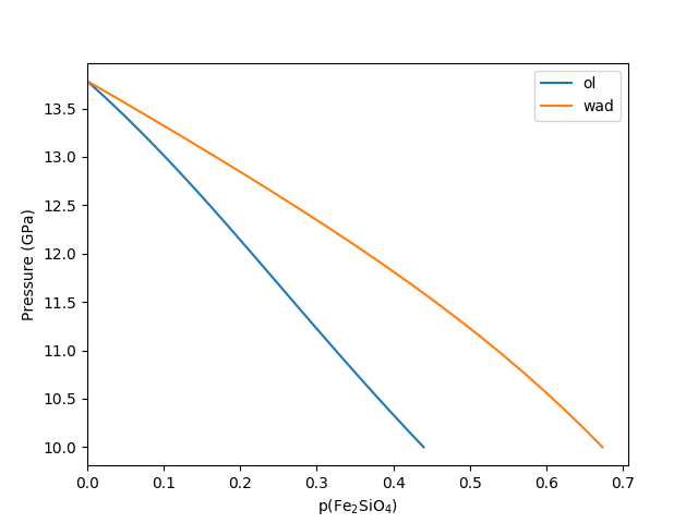
example_composite
This example demonstrates the functionalities of the burnman.Composite class.
Uses:
Demonstrates:
How to initialize a composite object containing minerals and solutions
How to set state and composition of composite objects
How to interrogate composite objects for their compositional, thermodynamic and thermoelastic properties.
How to use the stoichiometric and reaction affinity methods to solve simple thermodynamic equilibrium problems.
Please see example_equilibrate.py for more advanced (and user-friendly) examples of equilibration of a composite material.
Resulting figures:
example_calibrants
This example demonstrates the use of BurnMan’s library of pressure calibrants. These calibrants are stripped-down versions of BurnMan’s minerals, in that they are only designed to return pressure as a function of volume and temperature or volume as a function of pressure and temperature.
Uses:
burnman.calibrants.tools.pressure_to_pressure()Decker (1971) calibration for NaCl
Demonstrates:
Use of the Calibrant class
Conversion between pressures given by two different calibrations.
example_anisotropy
This example illustrates the basic functions required to convert an elastic stiffness tensor into elastic properties.
Specifically uses:
Demonstrates:
anisotropic functions
Resulting figure:
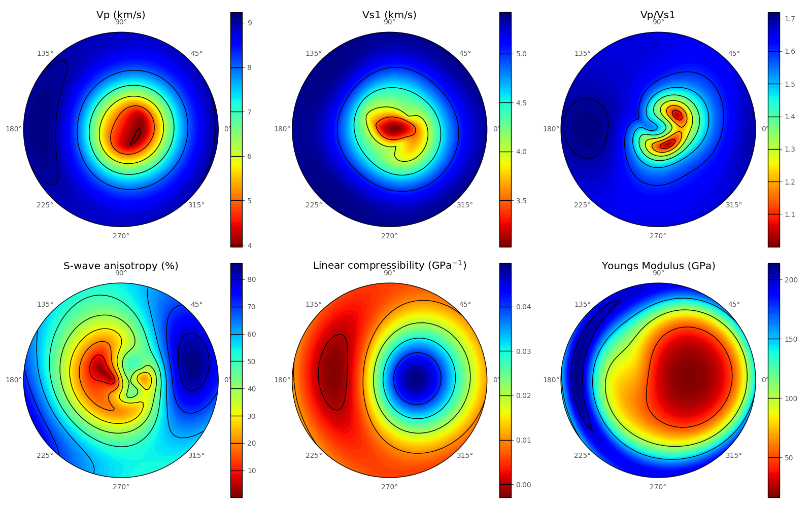
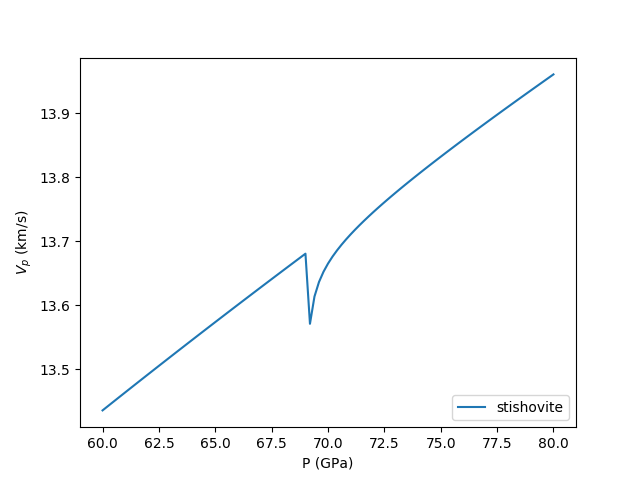
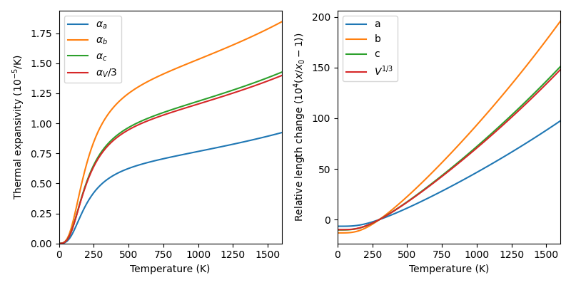
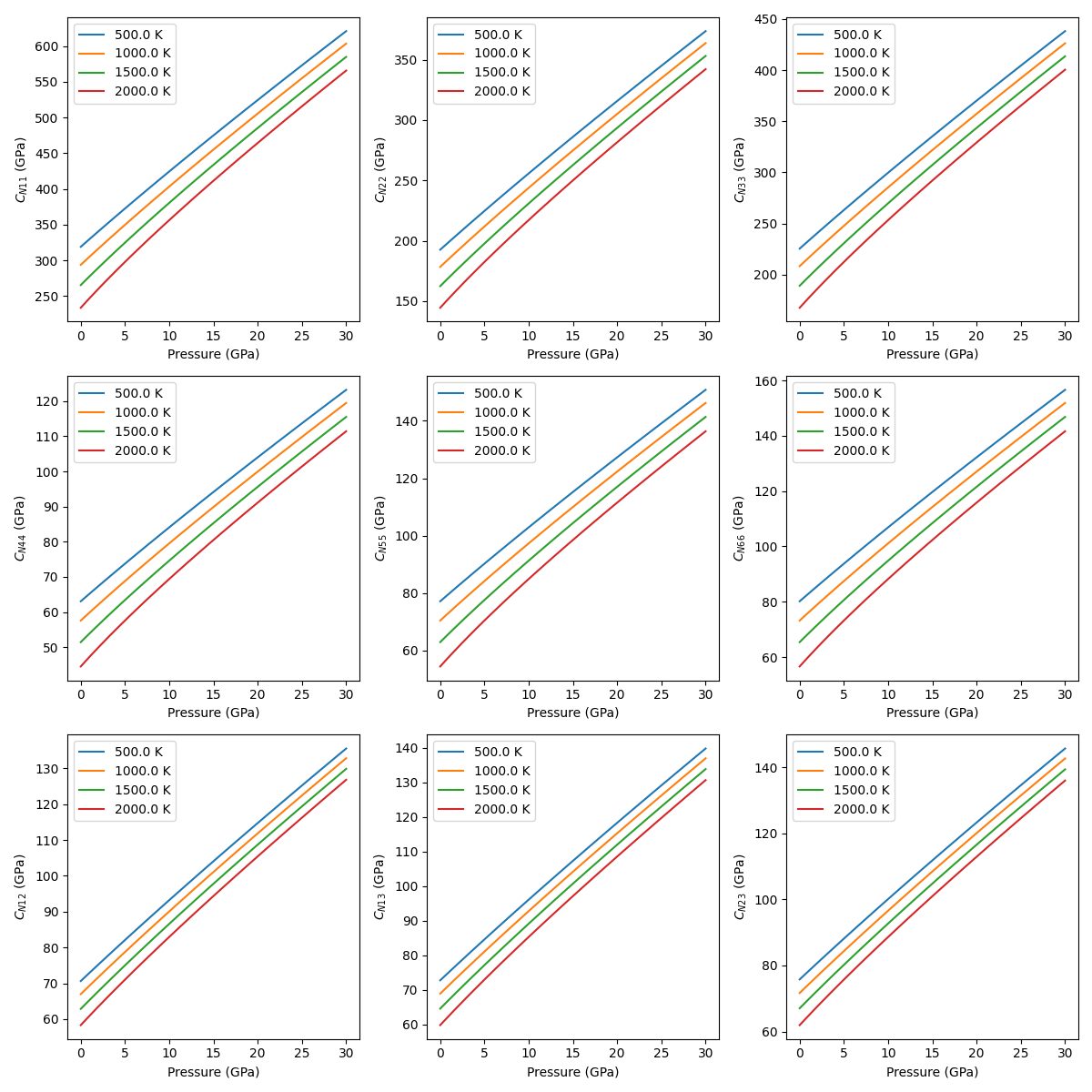
example_anisotropic_mineral
This example illustrates how to create and interrogate an AnisotropicMineral object.
Specifically uses:
Demonstrates:
anisotropic functions
Resulting figure:
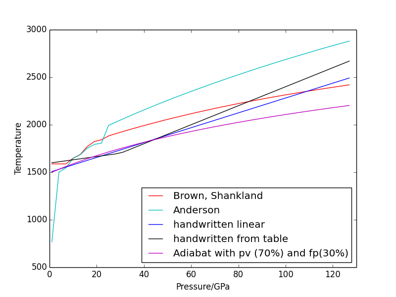
example_geotherms
This example shows each of the geotherms currently possible with BurnMan. These are:
Brown and Shankland, 1981 [BS81]
Anderson, 1982 [And82]
Stacey, 1977 continental [Sta77]
Stacey, 1977 oceanic [Sta77]
Custom tabulated geotherm
Adiabatic geotherm for a given mineral assemblage
Uses:
burnman.geotherm.BrownShankland
burnman.geotherm.Anderson
burnman.geotherm.StaceyContinental
burnman.geotherm.StaceyOceanic
burnman.geotherm.Geotherm
burnman.geotherm.AdiabaticGeotherm
burnman.Compositefor adiabatDemonstrates:
the available geotherms
Resulting figure:
example_composition
This example script demonstrates the use of BurnMan’s Composition class.
Uses:
Demonstrates:
Creating an instance of the Composition class with a molar or weight composition
Printing weight, molar, atomic compositions
Renormalizing compositions
Modifying the independent set of components
Modifying compositions by adding and removing components