Examples
BurnMan comes with a large collection of example programs under examples/. Below you can find a summary of the different examples. They are grouped into Simple Examples and More Advanced Examples. We suggest starting with the Tutorial before moving on to the examples, especially if you are new to using BurnMan.
Finally, we also include the scripts that were used for all computations and figures in the 2014 BurnMan paper in the misc/ folder, see Reproducing Cottaar, Heister, Rose and Unterborn (2014).
Simple Examples
- The following is a list of simple examples:
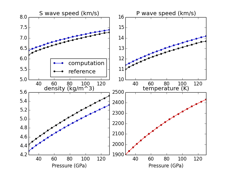
example_beginner
This example script is intended for absolute beginners to BurnMan. We cover importing BurnMan modules, creating a composite material, and calculating its seismic properties at lower mantle pressures and temperatures. Afterwards, we plot it against a 1D seismic model for visual comparison.
Uses:
Demonstrates:
creating basic composites
calculating thermoelastic properties
seismic comparison
Resulting figure:
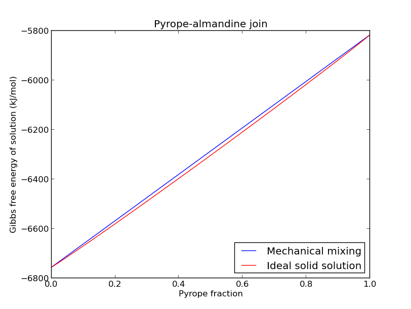
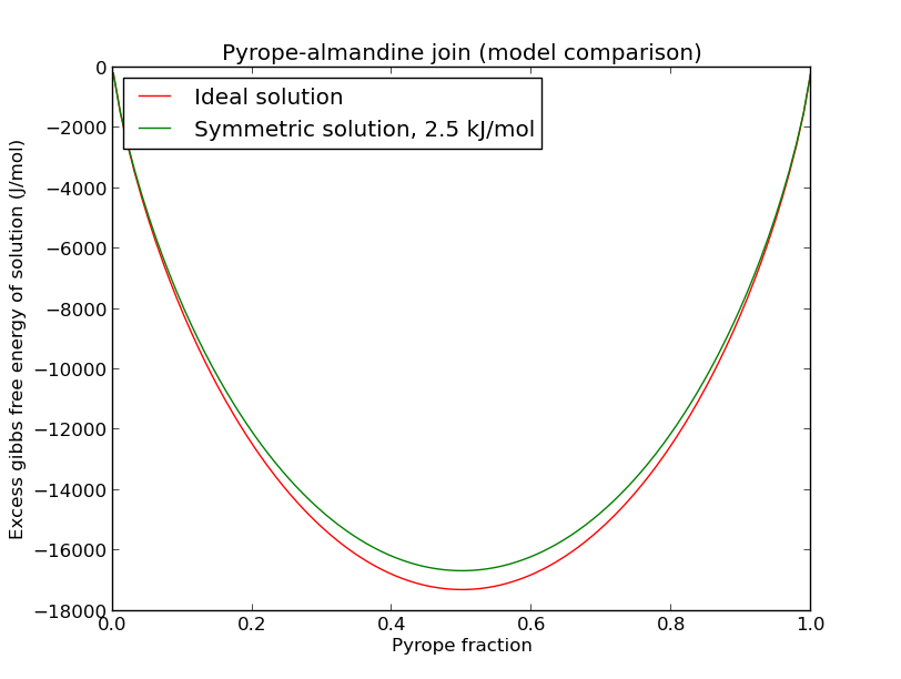
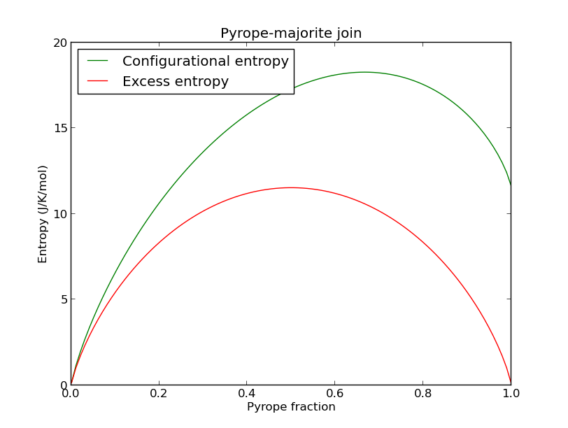
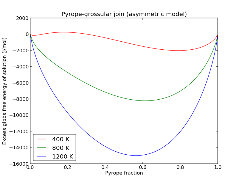
example_solid_solution
This example shows how to create different solid solution models and output thermodynamic and thermoelastic quantities.
There are four main types of solid solution currently implemented in BurnMan:
Ideal solid solutions
Symmmetric solid solutions
Asymmetric solid solutions
Subregular solid solutions
These solid solutions can potentially deal with:
Disordered endmembers (more than one element on a crystallographic site)
Site vacancies
More than one valence/spin state of the same element on a site
Uses:
Demonstrates:
Different ways to define a solid solution
How to set composition and state
How to output thermodynamic and thermoelastic properties
Resulting figures:
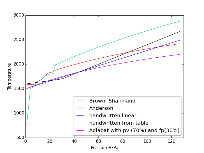
example_geotherms
This example shows each of the geotherms currently possible with BurnMan. These are:
Brown and Shankland, 1981 [BS81]
Anderson, 1982 [And82]
Watson and Baxter, 2007 [WB07]
linear extrapolation
Read in from file from user
Adiabatic from potential temperature and choice of mineral
Uses:
input geotherm file input_geotherm/example_geotherm.txt (optional)
burnman.composite.Compositefor adiabat
Demonstrates:
the available geotherms
Resulting figure:
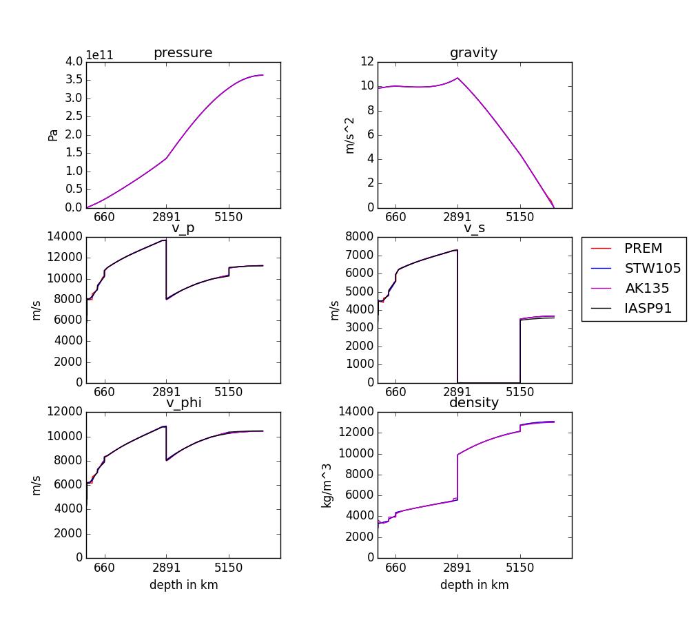
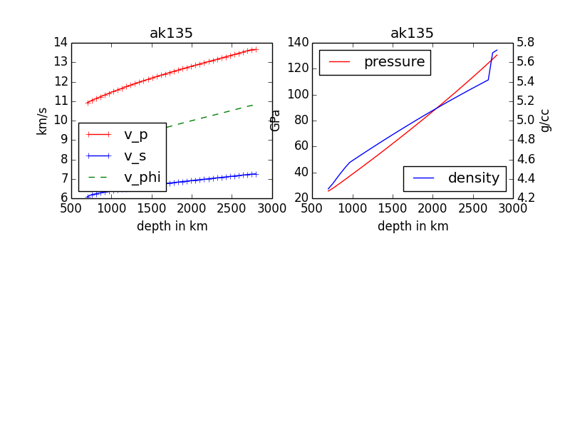
example_seismic
Shows the various ways to input seismic models (\(V_s, V_p, V_{\phi}, \rho\)) as a function of depth (or pressure) as well as different velocity model libraries available within Burnman:
This example will first calculate or read in a seismic model and plot the model along the defined pressure range. The example also illustrates how to import a seismic model of your choice, here shown by importing AK135 [KEB95].
Uses:
Demonstrates:
Utilization of library seismic models within BurnMan
Input of user-defined seismic models
Resulting figures:
example_composition
This example script demonstrates the use of BurnMan’s Composition class.
Uses:
burnman.composition.Composition
Demonstrates:
Creating an instance of the Composition class with a molar or weight composition
Printing weight, molar, atomic compositions
Renormalizing compositions
Modifying the independent set of components
Modifying compositions by adding and removing components
Resulting figure:
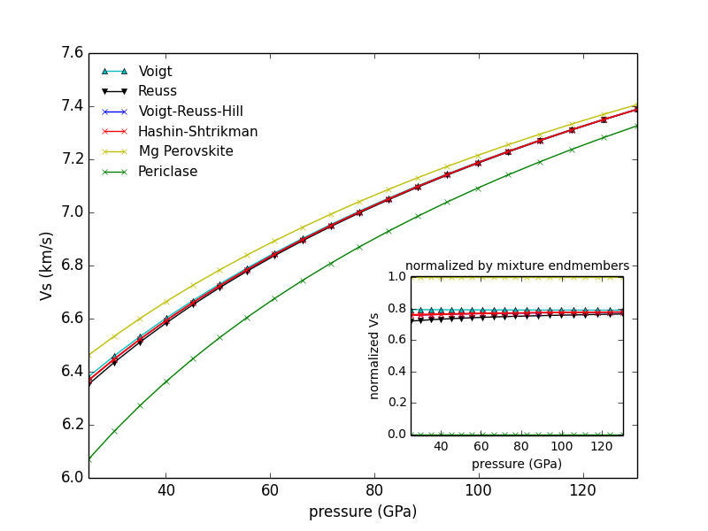
example_averaging
This example shows the effect of different averaging schemes. Currently four averaging schemes are available:
Voight-Reuss-Hill
Voight averaging
Reuss averaging
Hashin-Shtrikman averaging
See [WDOConnell76] Journal of Geophysics and Space Physics for explanations of each averaging scheme.
Specifically uses:
Demonstrates:
implemented averaging schemes
Resulting figure:
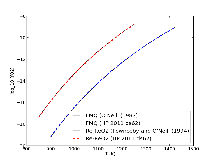
example_chemical_potentials
This example shows how to use the chemical potentials library of functions.
Demonstrates:
How to calculate chemical potentials
How to compute fugacities and relative fugacities
Resulting figure:
More Advanced Examples
- Advanced examples:
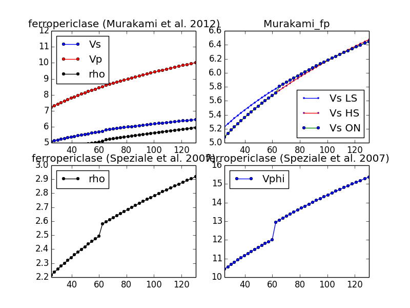
example_spintransition
This example shows the different minerals that are implemented with a spin transition. Minerals with spin transition are implemented by defining two separate minerals (one for the low and one for the high spin state). Then a third dynamic mineral is created that switches between the two previously defined minerals by comparing the current pressure to the transition pressure.
Specifically uses:
Demonstrates:
implementation of spin transition in (Mg,Fe)O at user defined pressure
Resulting figure:
example_user_input_material
Shows user how to input a mineral of his/her choice without usint the library and which physical values need to be input for BurnMan to calculate \(V_P, V_\Phi, V_S\) and density at depth.
Specifically uses:
Demonstrates:
how to create your own minerals
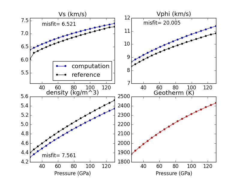
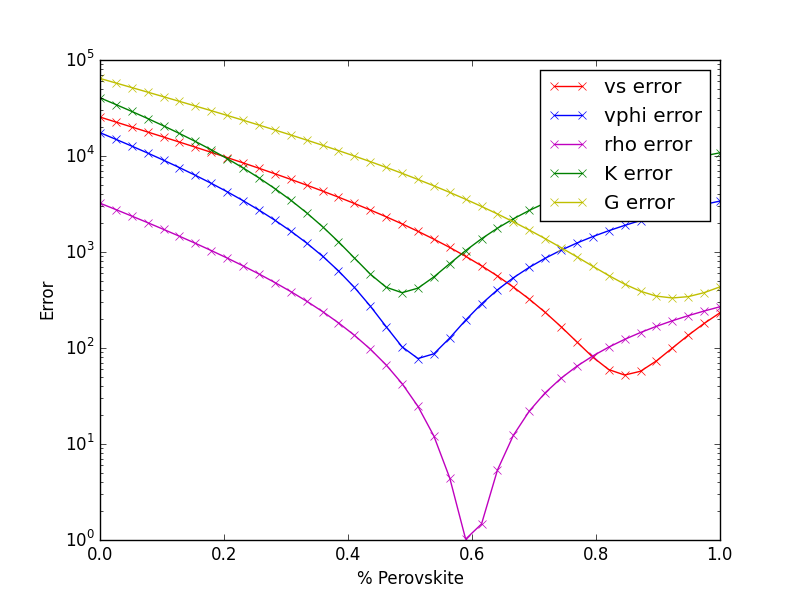
example_optimize_pv
Vary the amount perovskite vs. ferropericlase and compute the error in the seismic data against PREM. For more extensive comments on this setup, see tutorial/step_2.py
Uses:
Demonstrates:
compare errors between models
loops over models
Resulting figure:
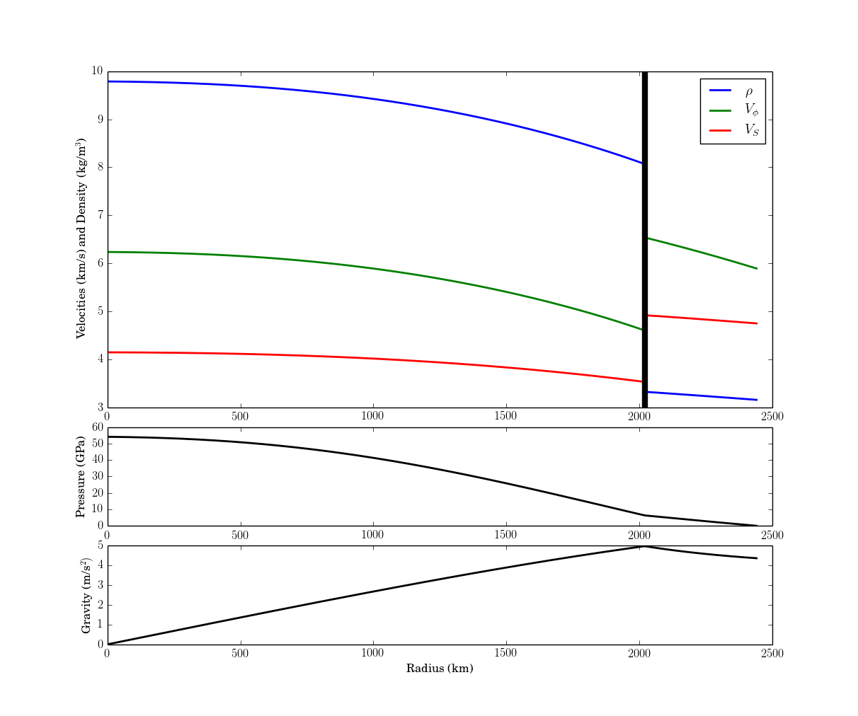
example_build_planet
For Earth we have well-constrained one-dimensional density models. This allows us to calculate pressure as a function of depth. Furthermore, petrologic data and assumptions regarding the convective state of the planet allow us to estimate the temperature.
For planets other than Earth we have much less information, and in particular we know almost nothing about the pressure and temperature in the interior. Instead, we tend to have measurements of things like mass, radius, and moment-of-inertia. We would like to be able to make a model of the planet’s interior that is consistent with those measurements.
However, there is a difficulty with this. In order to know the density of the planetary material, we need to know the pressure and temperature. In order to know the pressure, we need to know the gravity profile. And in order to the the gravity profile, we need to know the density. This is a nonlinear problem which requires us to iterate to find a self-consistent solution.
This example allows the user to define layers of planets of known outer radius and self- consistently solve for the density, pressure and gravity profiles. The calculation will iterate until the difference between central pressure calculations are less than 1e-5. The planet class in BurnMan (../burnman/planet.py) allows users to call multiple properties of the model planet after calculations, such as the mass of an individual layer, the total mass of the planet and the moment if inertia. See planets.py for information on each of the parameters which can be called.
Uses:
burnman.planet.Planet- class
burnman.layer.Layer
Demonstrates:
setting up a planet
computing its self-consistent state
computing various parameters for the planet
seismic comparison
Resulting figure:
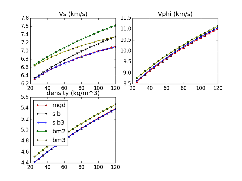
example_compare_all_methods
This example demonstrates how to call each of the individual calculation methodologies that exist within BurnMan. See below for current options. This example calculates seismic velocity profiles for the same set of minerals and a plot of \(V_s, V_\phi\) and \(\rho\) is produce for the user to compare each of the different methods.
Specifically uses:
Demonstrates:
Each method for calculating velocity profiles currently included within BurnMan
Resulting figure:
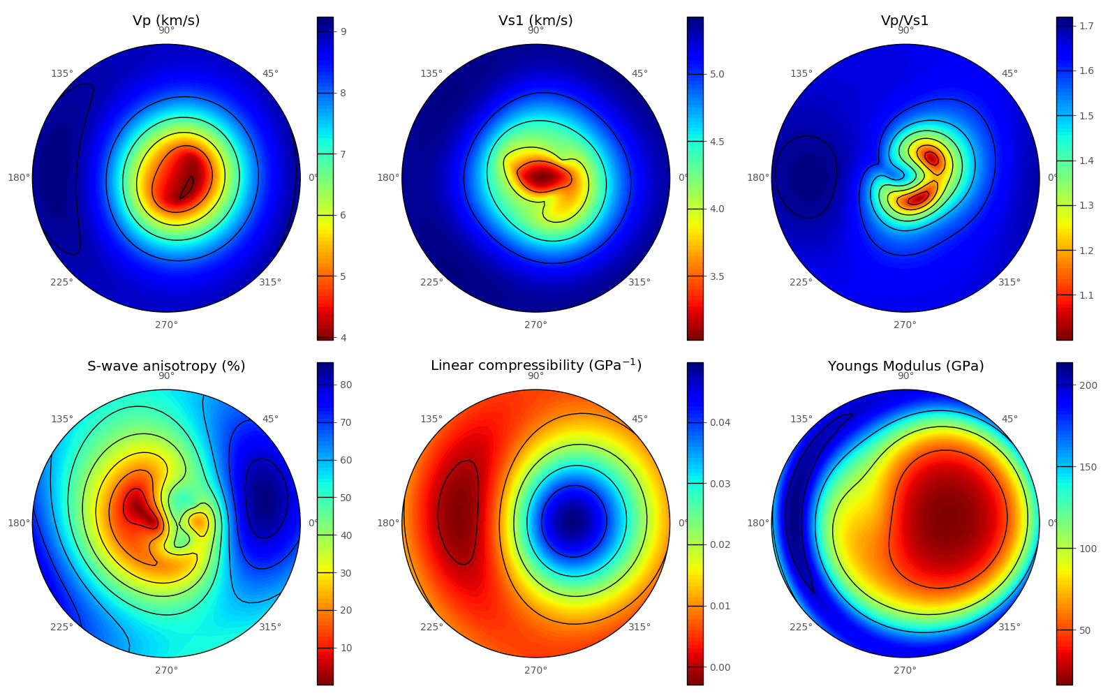
example_anisotropy
This example illustrates the basic functions required to convert an elastic stiffness tensor into elastic properties.
Specifically uses:
burnman.AnisotropicMaterial
Demonstrates:
anisotropic functions
Resulting figure:
example_fit_data
This example demonstrates BurnMan’s functionality to fit various mineral physics data to an EoS of the user’s choice.
Please note also the separate file example_fit_eos.py, which can be viewed as a more advanced example in the same general field.
teaches: - least squares fitting
Resulting figures:
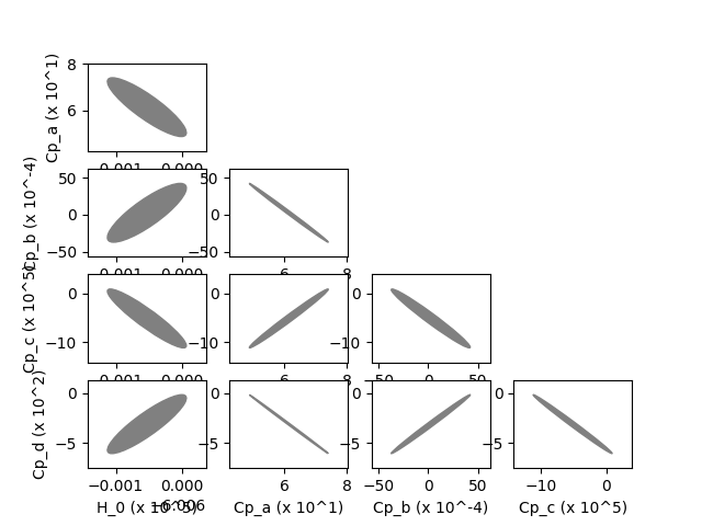
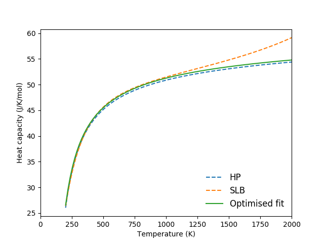
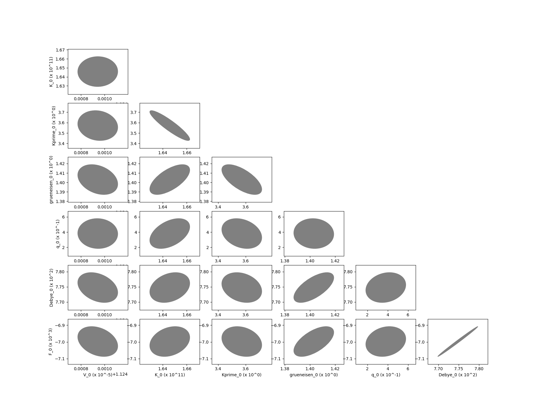
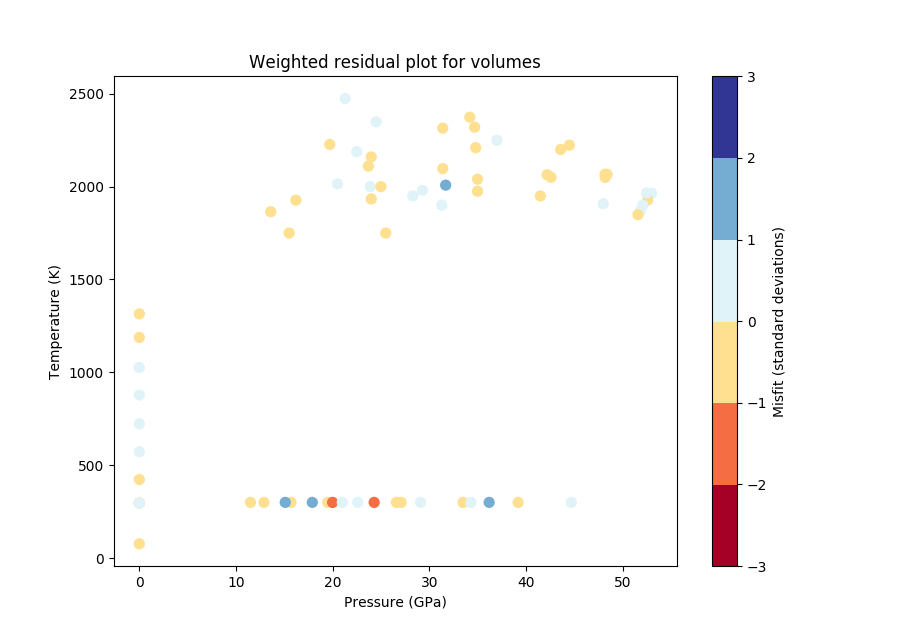
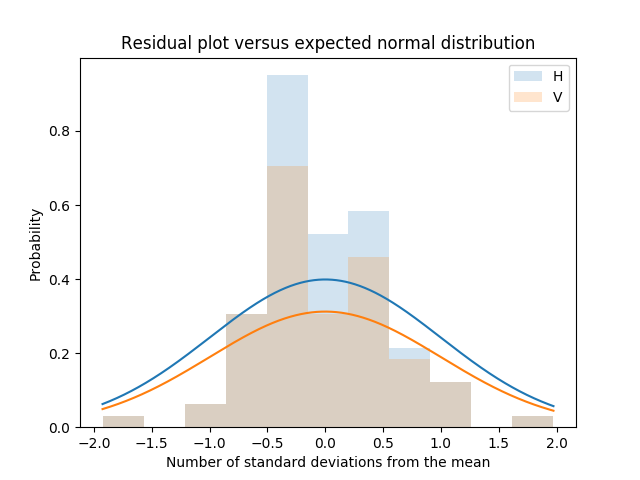
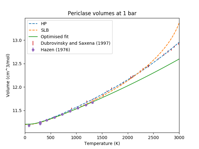
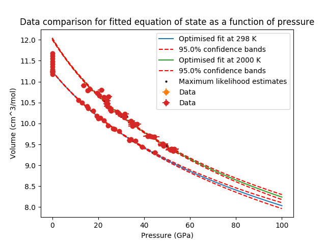
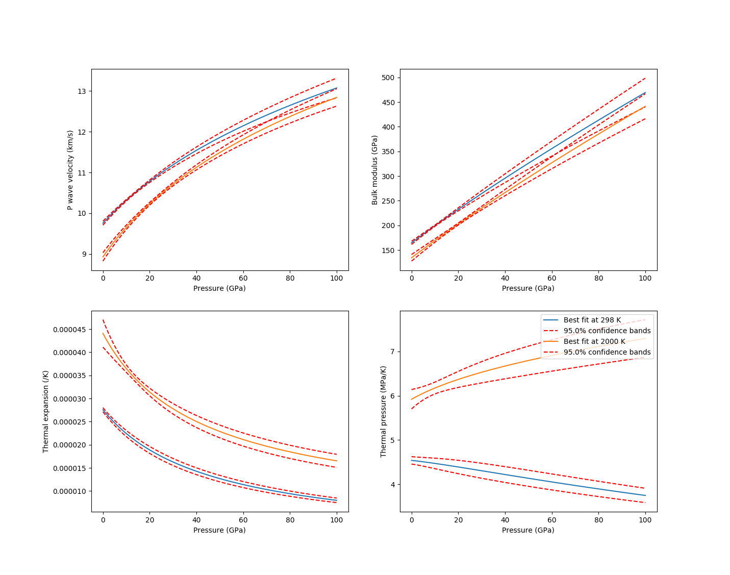
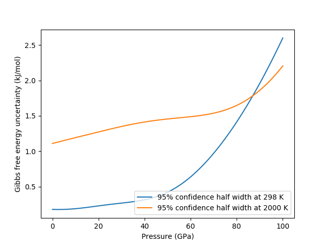
example_fit_eos
This example demonstrates BurnMan’s functionality to fit data to an EoS of the user’s choice.
The first example deals with simple PVT fitting. The second example illustrates how powerful it can be to provide non-PVT constraints to the same fitting problem.
teaches: - least squares fitting
Last seven resulting figures:
Reproducing Cottaar, Heister, Rose and Unterborn (2014)
In this section we include the scripts that were used for all computations and figures in the 2014 BurnMan paper: Cottaar, Heister, Rose & Unterborn (2014) [CHRU14]
paper_averaging
This script reproduces [CHRU14], Figure 2.
This example shows the effect of different averaging schemes. Currently four averaging schemes are available: 1. Voight-Reuss-Hill 2. Voight averaging 3. Reuss averaging 4. Hashin-Shtrikman averaging
See [WDOConnell76] for explanations of each averaging scheme.
requires: - geotherms - compute seismic velocities
teaches: - averaging
paper_benchmark
This script reproduces the benchmark in [CHRU14], Figure 3.
paper_fit_data
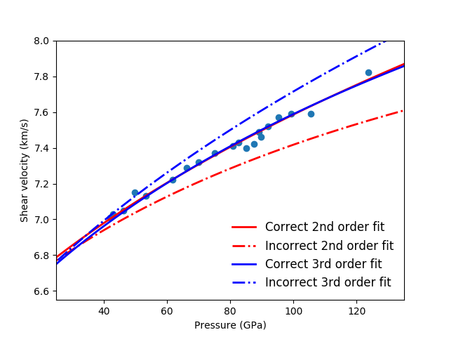
This script reproduces [CHRU14] Figure 4.
This example demonstrates BurnMan’s functionality to fit thermoelastic data to both 2nd and 3rd orders using the EoS of the user’s choice at 300 K. User’s must create a file with \(P, T\) and \(V_s\). See input_minphys/ for example input files.
requires: - compute seismic velocities
teaches: - averaging
paper_incorrect_averaging
This script reproduces [CHRU14], Figure 5. Attempt to reproduce Figure 6.12 from [Mur13]
paper_opt_pv
This script reproduces [CHRU14], Figure 6. Vary the amount perovskite vs. ferropericlase and compute the error in the seismic data against PREM.
requires: - creating minerals - compute seismic velocities - geotherms - seismic models - seismic comparison
teaches: - compare errors between models - loops over models
paper_onefit
This script reproduces [CHRU14], Figure 7. It shows an example for a best fit for a pyrolitic model within mineralogical error bars.
paper_uncertain
This script reproduces [CHRU14], Figure 8. It shows the sensitivity of the velocities to various mineralogical parameters.
Misc or work in progress
example_grid
This example shows how to evaluate seismic quantities on a \(P,T\) grid.
example_woutput
This example explains how to perform the basic i/o of BurnMan. A method of calculation is chosen, a composite mineral/material (see example_composition.py for explanation of this process) is created in the class “rock,” finally a geotherm is created and seismic velocities calculated.
Post-calculation, the results are written to a simple text file to plot/manipulate at the user’s whim.
requires: - creating minerals - compute seismic velocities - geotherms
teaches: - output computed seismic data to file